Sampling Variability

8.3. Sampling Variability#

In Section 8.1, we treated the 244 bills in the tips data as a sample from all the bills at a restaurant. A number computed from a sample, such as a sample mean or a sample proportion, is called a statistic. The number we really want, such as the mean of all bills, is a parameter of the population. Because a different sample would give a different statistic, every estimate carries some uncertainty. This section uses simulation to see how much statistics vary from sample to sample, and how sample size controls that variation.

8.3.1. Samples from a Known Population #

In real analyses we never see the whole population. To watch sampling variability happen, we flip the situation around: we treat the 244 bills as the entire population and draw small random samples from them. Then we know the true answer and can compare each sample to it.

The population mean is a parameter. We usually write it as $\mu$ (mu).

tips = sns.load_dataset('tips')
bills = tips['total_bill'].to_numpy()       ### the population: all 244 bills

mu = bills.mean()                           ### parameter: population mean
print('Population mean (mu):', round(mu, 2))

Population mean (mu): 19.79

Now draw a random sample of 20 bills and compute its mean. The sample mean, written $\bar x$ (x-bar), is a statistic. We sample with replacement, as if each bill were drawn at random from the restaurant’s steady stream of customers.

rng = np.random.default_rng(42)
n = 20

for i in range(3):
    sample = rng.choice(bills, size=n, replace=True)     ### one random sample of 20 bills
    print(f'Sample {i + 1} mean: {sample.mean():.2f}')

Sample 1 mean: 22.45
Sample 2 mean: 17.54
Sample 3 mean: 20.98

Each sample gives a different mean, and none of them equals $\mu$ exactly. That is sampling variability. To see its pattern, we repeat the process 5,000 times and plot all 5,000 sample means. The distribution of a statistic across repeated samples is called its sampling distribution.

n_sims = 5_000
sample_means = np.array([rng.choice(bills, size=n, replace=True).mean() for _ in range(n_sims)])

fig, ax = plt.subplots(1, 2, figsize=(11, 4))
sns.histplot(bills, bins=20, color="#bab0ac", ax=ax[0])
ax[0].axvline(mu, color="black", linestyle=":", label="population mean")
ax[0].set(xlabel="total bill ($)", title="Population: 244 bills")
ax[0].legend()

sns.histplot(sample_means, bins=30, color="#4c78a8", ax=ax[1])
ax[1].axvline(mu, color="black", linestyle=":", label="population mean")
ax[1].set(xlabel="sample mean ($)", title=f"5,000 sample means (n = {n})")
ax[1].legend()
plt.tight_layout()
plt.show()

print('Mean of the sample means:', round(sample_means.mean(), 2))
print('SD of the sample means:  ', round(sample_means.std(ddof=1), 2))

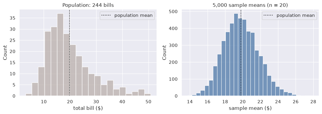
../../_images/96b94227b54a7c78961b4b45f46e5b1a9612e4903e86733d9ffbeb89b49bb47f.png

Mean of the sample means: 19.78
SD of the sample means:   1.99

Three things stand out:

Center: the sample means are centered on the population mean. Any single sample can miss, but on average the sample mean hits the target.
Spread: the sample means vary much less than individual bills. Averaging 20 bills cancels out many of the high and low values.
Shape: the bills themselves are skewed to the right, but the sample means form a roughly symmetric, bell-shaped distribution. This is the Central Limit Theorem from Section 8.2, now applied to sample means.

The SD of the sample means measures how far a sample mean typically lands from $\mu$. It has its own name, the standard error, which we return to below.

8.3.2. Simulating Sample Proportions #

The same idea works for proportions. Suppose 60% of a store’s customers use a loyalty card. Each customer is like a flip of a weighted coin that comes up “yes” with probability $p = 0.6$. We simulate many samples of customers to see how the sample proportion varies.

Key quantities:

True proportion $p$ (a parameter)
Sample size $n$
Sample proportion $\hat p$ (a statistic)
Sampling distribution: distribution of $\hat p$ across repeated samples

rng = np.random.default_rng(seed=0)

p_true = 0.6
n = 40
n_sims = 5_000

# Draw many samples and compute sample proportions
samples = rng.binomial(n=n, p=p_true, size=n_sims)      # Draw samples from a binomial distribution
sample_props = samples / n                              # Compute sample proportions    

summary = pd.Series(sample_props).describe(percentiles=[0.025, 0.5, 0.975]).round(3)
summary

count    5000.000
mean        0.600
std         0.078
min         0.350
2.5%        0.450
50%         0.600
97.5%       0.750
max         0.850
dtype: float64

We see that

97.5% of the simulated sample proportions fell at or below 0.750.
2.5%, the lower bound, is 0.450.
the middle 95% of simulated proportions fall between 0.45 and 0.75.

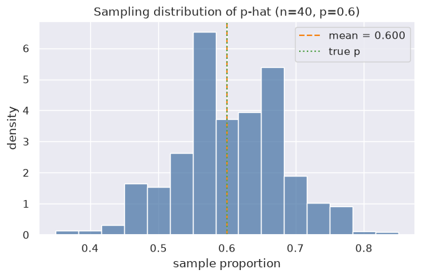
Now let us take a look at the sampling distribution: the distribution of sample proportions (sample_props) generated from 5,000 simulated samples.

8.3.3. Sampling Distribution #

fig, ax = plt.subplots(figsize=(7, 4))
sns.histplot(sample_props, bins=15, stat="density", color="#4c78a8", edgecolor="white", ax=ax)

ax.axvline(sample_props.mean(), color="#f58518", linestyle="--", label=f"mean = {sample_props.mean():.3f}")
ax.axvline(p_true, color="#54a24b", linestyle=":", label="true p")
ax.set(xlabel="sample proportion", ylabel="density", title="Sampling distribution of p-hat (n=40, p=0.6)")
ax.legend()
plt.show()

../../_images/785469141cd9e1dd60d7dd226feb48abc7761db876e60b6d33c5db63e9fa97ac.png

8.3.3.1. Two Levels: the Data and the Samples #

It is easy to mix up two different distributions here:

	One survey’s data	The sampling distribution
What is in it	40 yes/no answers from one sample of customers	5,000 values of $\hat p$, one from each simulated survey
Summarized by	one number, $\hat p$	its center and spread (the standard error)
Where it comes from	what a company actually collects	imagined, or simulated

The histogram above shows the sampling distribution: each bar counts surveys, not customers. A company only ever runs one survey, so it sees one $\hat p$. The sampling distribution tells it how far that one number might be from the truth.

8.3.4. Standard Error #

For a sample proportion, the standard error measures the typical deviation of $\hat p$ from $p$:

\[\text{SE}(\hat p) = \sqrt{\dfrac{p(1-p)}{n}}\]

The SE is “sampling variability” expressed as a single number: it is the standard deviation of the sampling distribution of $\hat p$. Here $p = 0.6$ is the true proportion (a parameter), and $\hat p$ is the proportion observed in one sample (a statistic).

Note that:

$p(1-p)$ is the variance of a single yes/no observation. It is largest at $p = 0.5$ (most uncertain) and shrinks as $p$ approaches 0 or 1. For example, if $p = 0.6$, then $0.6 \times 0.4 = 0.24$.
Plug in $\hat p$: in real data analysis you don’t know $p$ (that’s why you’re sampling!), so you substitute the observed $\hat p$ into the formula. It’s an approximation, but it works well for reasonably large $n$.

Here we compare the empirical SD of simulations vs. the theoretical SE, to confirm that they match. In the comparison below, ddof stands for Delta Degrees of Freedom. It controls the denominator used in the std calculation. If ddof=0, divides by n (population std); if ddof=1, divides by n−1 (sample std).

The theoretical SE is the formula applied to the known values:
```
sqrt(0.6 × (1-0.6) / 40) ≈ 0.0775.
```
The empirical SE is the standard deviation of the 5,000 simulated p-hat values – no formula, purely from the simulation.
If the theoretical SE comes out nearly identical with the empirical (simulation) SE, then it validates that the formula is correct and the simulation is working as expected.

se_theoretical = np.sqrt(p_true * (1 - p_true) / n)
se_empirical = sample_props.std(ddof=1)

print(f"Theoretical SE: {se_theoretical:.4f}")
print(f"Simulated SE:   {se_empirical:.4f}")

Theoretical SE: 0.0775
Simulated SE:   0.0781

8.3.4.1. Margin of Error #

The sampling distribution of $\hat p$ is roughly normal, so the 68–95–99.7 rule from Section 8.2 applies: about 95% of sample proportions land within 2 standard errors of $p$. Two standard errors is the margin of error, the “plus or minus” reported with surveys and polls.

moe = 2 * se_theoretical
print(f"Margin of error (2 SE): {moe:.3f}")
print(f"p ± 2 SE: {p_true - moe:.3f} to {p_true + moe:.3f}")
print("Simulated middle 95%:", np.percentile(sample_props, [2.5, 97.5]))

Margin of error (2 SE): 0.155
p ± 2 SE: 0.445 to 0.755
Simulated middle 95%: [0.45 0.75]

The range $0.6 \pm 0.155$, or about 0.445 to 0.755, matches the middle 95% of the 5,000 simulated proportions (0.45 to 0.75).

Worked example. In practice we do not know $p$. Suppose a survey of 40 customers finds that 26 would renew, so $\hat p = 26/40 = 0.65$. Plugging in $\hat p$:

p_hat = 26 / 40
se_hat = np.sqrt(p_hat * (1 - p_hat) / 40)

print(f"p-hat: {p_hat:.2f}")
print(f"SE: {se_hat:.4f}")
print(f"Plausible range for p: {p_hat - 2 * se_hat:.2f} to {p_hat + 2 * se_hat:.2f}")

p-hat: 0.65
SE: 0.0754
Plausible range for p: 0.50 to 0.80

The true share of customers who would renew is plausibly anywhere from about 50% to 80%. A survey of 40 cannot tell a manager whether “half” or “four out of five” customers will renew. If the decision depends on that difference, the company needs a larger sample. Chapter 11 turns this idea into confidence intervals.

8.3.4.2. SE of a Sample Mean #

The sample mean has a standard error formula too. If the population has standard deviation $\sigma$ (sigma), the standard error of the mean of $n$ observations is

\[\text{SE}(\bar x) = \dfrac{\sigma}{\sqrt{n}}\]

Let us check it against the tips simulation from the start of this section. Because the 244 bills are the whole population, we use the population SD, np.std() with its default ddof=0.

sigma = np.std(bills)                                  ### population SD of the 244 bills
se_mean_formula = sigma / np.sqrt(20)
se_mean_sim = sample_means.std(ddof=1)                 ### SD of the 5,000 simulated sample means

print(f"Population SD (sigma): {sigma:.2f}")
print(f"SE formula, n = 20:    {se_mean_formula:.2f}")
print(f"Simulated SE:          {se_mean_sim:.2f}")

Population SD (sigma): 8.88
SE formula, n = 20:    1.99
Simulated SE:          1.99

The formula and the simulation agree. Individual bills vary by about $8.88, but means of 20 bills vary by only about $2. As with proportions, in practice we do not know $\sigma$, so we plug in the sample SD $s$ and use $s / \sqrt{n}$.

8.3.5. Effect of Sample Size #

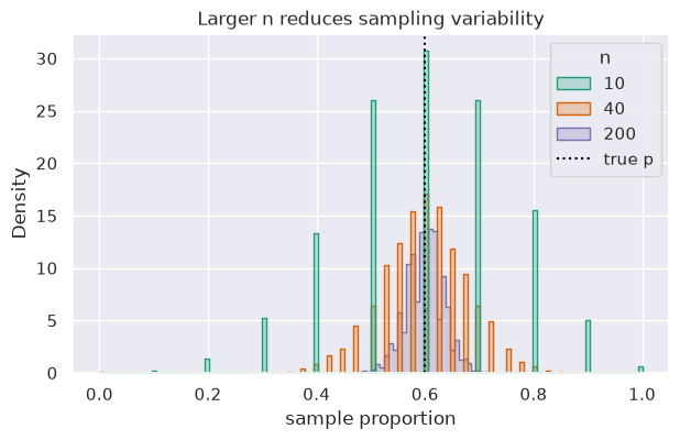
Larger samples shrink variability. Below we compare sampling distributions (p-hats) across different $n$ while keeping $p=0.6$ fixed.

def simulate_props(n, p=0.6, sims=5_000):
    props = rng.binomial(n=n, p=p, size=sims) / n   # Simulate sample proportions by drawing from a binomial distribution and dividing by n
    return props

ns = [10, 40, 200]
records = []
frames = []
for n_i in ns:
    props_i = simulate_props(n=n_i)
    frames.append(pd.DataFrame({"n": n_i, "prop": props_i}))    # Store the sample proportions in a DataFrame for plotting
    records.append({
        "n": n_i,
        "mean(p-hat)": props_i.mean(),
        "sd(p-hat)": props_i.std(ddof=1),
        "SE formula": np.sqrt(p_true * (1 - p_true) / n_i)
    })

display(pd.DataFrame(records).round(4))

plot_df = pd.concat(frames, ignore_index=True)
fig, ax = plt.subplots(figsize=(7, 4))
sns.histplot(data=plot_df, x="prop", hue="n", element="step", stat="density", common_norm=False, palette="Dark2", ax=ax)
vline = ax.axvline(p_true, color="black", linestyle=":")
ax.set(xlabel="sample proportion", title="Larger n reduces sampling variability")

leg = ax.get_legend()
handles = list(leg.legend_handles) + [vline]
labels = [t.get_text() for t in leg.get_texts()] + ["true p"]
ax.legend(handles=handles, labels=labels, title="n")
plt.show()

	n	mean(p-hat)	sd(p-hat)	SE formula
0	10	0.5994	0.1549	0.1549
1	40	0.5984	0.0780	0.0775
2	200	0.5986	0.0348	0.0346

../../_images/48b8b10270b0156721011b1ae88e77b44682b096871211015f26852e146a4698.png

Common mistakes

Confusing SD and SE. The standard deviation describes how much individual values vary (single bills vary by about $8.88). The standard error describes how much an estimate varies from sample to sample (means of 20 bills vary by about $2). Use the SD to describe data and the SE to describe the precision of a statistic.
Thinking a bigger sample fixes a biased one. The standard error assumes a random sample. If a company surveys only customers who use its app, a sample of 10,000 gives a very precise estimate of the wrong thing. Sample size reduces chance error, not bias.
Thinking a bigger population needs a bigger sample. The SE formula depends on the sample size $n$, not on the size of the population. A random sample of 1,000 is about as precise for a city as for a whole country.
The gambler’s fallacy. The law of large numbers does not mean that results “even out” in the short run. After five tails in a row, the next fair coin flip is still 50–50; the long-run average settles because later flips swamp the early ones, not because chance corrects itself.

Takeaways

Repeated samples vary; summarizing their distribution clarifies how much.
Standard error captures typical sampling fluctuation and shrinks as $n$ grows.
Simulations help check formulas and build intuition about variability.

As $n$ gets larger, the $\hat p$ values from repeated samples cluster more tightly around the true $p$. In the plot, the histogram for $n = 200$ is much narrower than for $n = 10$: the same true $p = 0.6$, but larger samples give estimates that are consistently closer to it.

The SE formula shows why: $\text{SE} = \sqrt{p(1-p)/n}$, so as $n$ increases, the SE decreases. Because $n$ is under a square root, quadrupling the sample size only cuts the SE in half. A larger sample gives you more information, so your estimate is less noisy. The SE turns the uncertainty in an estimate into a number a manager can use: a survey of 200 customers pins down the true proportion much more tightly than a survey of 10.

8.3.6. Section Practice #

Use this short exercise to check the main workflow from this section.

### Exercise: Practice Sampling Variability
# About 30% of a bank's customers use mobile check deposit. The bank plans a survey.
# The standard error of a sample proportion is sqrt(p * (1 - p) / n).
#   1. Compute the standard error for samples of 100 and of 900 customers.
#   2. How many times smaller is the standard error with 900 customers?
#   3. Print the two standard errors (3 decimals) and the ratio (1 decimal).
#   4. A survey of 100 customers finds that 27 of them use mobile deposit.
#      Is 0.27 a parameter or a statistic? Store the word in `kind`.
#   5. Deposit amounts have a standard deviation of $400. Compute the standard
#      error of the mean deposit, sd / sqrt(n), for n = 100 and n = 400.
# Print exactly:
# SE with n=100: 0.046
# SE with n=900: 0.015
# Ratio: 3.0
# 0.27 is a: statistic
# SE of mean deposit, n=100: 40.0
# SE of mean deposit, n=400: 20.0
import numpy as np

p = 0.3
sd_deposit = 400
### Your code starts here




### Your code ends here

SE with n=100: 0.046
SE with n=900: 0.015
Ratio: 3.0
0.27 is a: statistic
SE of mean deposit, n=100: 40.0
SE of mean deposit, n=400: 20.0

	One survey’s data	The sampling distribution
What is in it	40 yes/no answers from one sample of customers	5,000 values of \(\hat p\), one from each simulated survey
Summarized by	one number, \(\hat p\)	its center and spread (the standard error)
Where it comes from	what a company actually collects	imagined, or simulated

Sampling Variability

Contents

8.3. Sampling Variability#