
9.3. Hypotheses and p-Value#
The statistical and computational methodology that we developed for assessing models of jury selection fits into a general framework of decision making called statistical tests of hypotheses. Using statistical tests as a way of making decisions is standard in many fields and has a standard terminology.
In this section, we will outline the general sequence of steps used in statistical tests, along with some key terminology.
Though our example is from the biological sciences, you will see that the statistical and computational steps in the process are consistent with the corresponding steps in our analyses of data from the legal system. However, the biological data pertain to plants, not human beings, and do not raise the same concerns about injustice. So the context and interpretation of the calculations below are far simpler.
Run the demonstration cells in order. Use the comparison below to connect the three cases before learning the formal terms.
Case |
Null model |
Statistic |
Evidence against the model |
|---|---|---|---|
Swain |
Random draws with 26% Black panelists |
Count among 100 |
Unusually small counts |
Alameda |
Random draws with the stated eligible shares |
TVD between sample and eligible shares |
Unusually large distances |
Mendel |
Independent plants with 75% purple flowers |
Absolute distance from 75% |
Unusually large distances |
All three compare an observed statistic with a distribution generated under a stated model. The cases differ in what the statistic measures and which outcomes count as more extreme.
Gregor Mendel (1822-1884) was an Austrian monk who is widely recognized as the founder of the modern field of genetics. Mendel performed careful and large-scale experiments on plants to come up with fundamental laws of genetics.
Many of his experiments were on varieties of pea plants. He formulated sets of assumptions about each variety; these were his models. He then tested the validity of his models by growing the plants and gathering data.
For pea plants of a particular variety, Mendel proposed the following model.
9.3.1. Case 3: Mendel’s Experiment#
For every plant, there is a 75% chance that it will have purple flowers, and a 25% chance that the flowers will be white, regardless of the colors in all the other plants.
To see whether his model was valid, Mendel grew 929 pea plants of this variety. Among these 929 plants, 705 had purple flowers.
We will use these data to perform a test of hypotheses and see whether the data are consistent with Mendel’s model.
9.3.2. Step 1: The Hypotheses#
A statistical test assesses evidence against a specified view of how the data were generated. Specifically, the choice is between two views about how the data were generated. These two views are called hypotheses.
The null hypothesis. This is a clearly defined model about chances. It says that the data were generated at random under clearly specified assumptions about the randomness. The word “null” reinforces the idea that if the data look different from what the null hypothesis predicts, the difference is due to nothing but chance.
From a practical perspective, the null hypothesis is a hypothesis under which you can simulate data.
In the example about Mendel’s model for the colors of pea plants, the null hypothesis is that the assumptions of his model are good: each plant has a 75% chance of having purple flowers, independent of all other plants.
Under this hypothesis, we were able to simulate random samples, by using sample_proportions(929, [0.75, 0.25]). We used a sample size of 929 because that’s the number of plants Mendel grew.
The alternative hypothesis. This says that some reason other than chance made the data differ from the predictions of the model in the null hypothesis.
In the example about Mendel’s plants, the alternative hypothesis is simply that his model isn’t good.
Keep in mind that the alternative doesn’t say how or why the model isn’t good. It just says the model isn’t good.
For Mendel, write the claims as null: the probability of purple flowers is 0.75, with independent plants, and alternative: that probability differs from 0.75. The alternative allows either direction, so this is a two-sided test.
A manager asking only whether a defect rate has increased would instead use a one-sided alternative. Choose the direction from the question before examining the result. An unexpected decrease and an unexpected increase answer different management questions.
9.3.3. Step 2: The Test Statistic#
In order to decide between the two hypotheses, we must choose a statistic that we can use to make the decision. This is called the test statistic.
If the model is good, the percent of purple-flowering plants in the sample should be close to 75%. If the model is not good, the percent purple-flowering will be away from 75%. It may be higher, or lower; the direction doesn’t matter.
The key for us is the distance between 75% and the percent of purple-flowering plants in the sample. Big distances are evidence that the model isn’t good.
Our statistic, therefore, is the distance between the sample percent and 75%:
This test statistic is a distance between the two distributions. It makes sense and is easy to use. A sample percent of around 75% will be consistent with the model, but percents much bigger or much less than 75 will make you think that the model isn’t good. Therefore, small values of the distance will make you lean towards the null hypothesis. Big values of the statistic will make you lean towards the alternative.
To choose a test statistic in other situations, look at the alternative hypothesis. What values of the statistic will make you think that the alternative hypothesis is a better choice than the null?
If the answer is “big values,” you have a good choice of statistic.
So also if the answer is “small values.”
But if the answer is “both big values and small values,” we recommend that you look again at your statistic. See if using a distance instead of a difference can change the answer to just “big values”.
In the case of the pea plants, a sample percent of around 75% will be consistent with the model, but percents much bigger or much less than 75 will make you think that the model isn’t good. This indicates that the statistic should be the distance between the sample percent and 75, that is, the absolute value of the difference between them. Big values of the distance will make you lean towards the alternative.
Observed Value of the Test Statistic
The observed value of the test statistic is the value of the statistic you get from the data in the study, not a simulated value. Among Mendel’s 929 plants, 705 had purple flowers. The observed value of the test statistic was therefore
Taking an absolute distance folds both directions into one nonnegative statistic: 70% and 80% purple flowers are both five percentage points from 75%. Therefore, large distances form the right tail even though the alternative is two-sided. For a one-sided claim about an increase, a signed difference would retain the direction instead.
Check your reasoning: A test statistic is a rule you could apply to any sample. The observed statistic is the single value obtained by applying that rule to the real data.
observed_statistic = abs ( 100 * (705 / 929) - 75)
observed_statistic
0.8880516684607045
9.3.4. Step 3: The Distribution of the Test Statistic, Under the Null Hypothesis#
The main computational aspect of a test of hypotheses is figuring out what the model in the null hypothesis predicts. Specifically, we have to figure out what the values of the test statistic might be if the null hypothesis were true.
The test statistic is simulated based on the assumptions of the model in the null hypothesis. That model involves chance, so the statistic comes out differently when you simulate it multiple times.
By simulating the statistic repeatedly, we get a good sense of its possible values and which ones are more likely than others. In other words, we get a good approximation to the probability distribution of the statistic, as predicted by the model in the null hypothesis.
As with all distributions, it is very useful to visualize this distribution by a histogram, as we have done in our previous examples.
mendel_proportions = np.array([0.75, 0.25])
mendel_proportion_purple = mendel_proportions.item(0)
sample_size = 929
Next, we will define a function that returns one simulated value of the test statistic. Then we will use a for loop to collect 10,000 simulated values in an array.
def sample_proportions(sample_size, probabilities):
    """Return the proportion of random draws for each outcome in a distribution.
    This function is similar to np.random.multinomial, but returns proportions
    instead of counts.
    Args:
        ``sample_size``: The size of the sample to draw from the distribution.
        ``probabilities``: An array of probabilities that forms a distribution.
    Returns:
        An array with the same length as ``probability`` that sums to 1.
    """
    return np.random.multinomial(sample_size, probabilities) / sample_size
    # return np.random.multinomial(sample_size, probabilities)
def one_simulated_distance():
    sample_proportion_purple = sample_proportions(929, mendel_proportions).item(0)
    return 100 * abs(sample_proportion_purple - mendel_proportion_purple)
np.random.seed(42)
repetitions = 10000
distances = np.array([])
for i in np.arange(repetitions):
    distances = np.append(distances, one_simulated_distance())
Now we can draw the histogram of these values. This is the histogram of the distribution of the test statistic predicted by the null hypothesis.
pd.DataFrame({
    'Distance between Sample % and 75%': distances
}).hist( edgecolor='white', figsize=(5, 4))

plt.title('Prediction Made by the Null Hypothesis')
plt.xlabel('Distance between Sample % and 75%')
plt.ylabel('Count')
# plt.tight_layout()
Text(0, 0.5, 'Count')
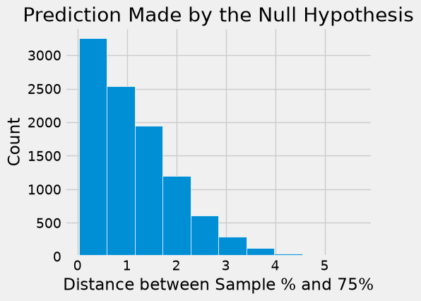
Look on the horizontal axis to see the typical values of the distance, as predicted by the model. They are rather small. For example, a high proportion of the distances are in the range 0 to 1, meaning that for a high proportion of the samples, the percent of purple-flowering plants is in the range 75% \(\pm\) 1%. That is, the sample percent is in the range 74% to 76%.
Also note that this prediction was made using Mendel’s model only, not the proportions observed by Mendel in the plants that he grew. It is time now to compare the predictions and Mendel’s observation.
9.3.5. Step 4. The Conclusion of the Test#
The choice between the null and alternative hypotheses depends on the comparison between what you computed in Steps 2 and 3: the observed value of the test statistic and its distribution as predicted by the null hypothesis.
If the two are not consistent with each other, then the data give evidence against the null hypothesis. We say that the test rejects the null hypothesis in favor of the alternative.
If the two are consistent with each other, then the observed test statistic is in line with what the null hypothesis predicts, and the data give no evidence against it. We say that the data are consistent with the null hypothesis, or that the test does not reject the null hypothesis.
Not rejecting is not the same as proving the null hypothesis true. Other models might fit the data just as well (a 74% or 76% chance of purple flowers, for example), and a small sample may simply not contain enough evidence to detect a real difference. That is why a test either rejects the null hypothesis or does not reject it; it never “accepts” the null.
In our example, the observed value of the test statistic is about 0.89, as computed in Step 2 above. Just by eye, locate roughly where 0.89 is on the horizontal axis of the histogram. You will see that it is clearly in the heart of the distribution predicted by Mendel’s model.
The cell below redraws the histogram with the observed value plotted on the horizontal axis.
fig, ax = plt.subplots(figsize=(6, 4))
ax.hist(distances, bins=np.arange(0, 6.25, 0.25), density=True, edgecolor='white')
ax.axvline(observed_statistic, color='red', linestyle='--', label='Observed distance')
ax.set_title('Prediction Made by the Null Hypothesis')
ax.set_xlabel('Distance from 75% (Percentage Points)')
ax.set_ylabel('Probability Density')
ax.legend()
<matplotlib.legend.Legend at 0x7f8f80dfba10>
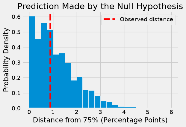
The observed statistic is like a typical distance predicted by the null hypothesis. The null hypothesis is Mendel’s model. So our test concludes that the data are consistent with Mendel’s model.
Based on our data, the test does not reject Mendel’s model. That does not prove the model is right; it means these 929 plants give no evidence against it.
9.3.6. The Meaning of “Consistent”#
The jury-panel observations were far from the values typically predicted by their models. Mendel’s observed distance was much more typical. Other observations may be harder to judge from a graph alone.
A significance level, often written as alpha, is a cutoff for a decision rule. Choose the null model, alternative, statistic, and cutoff before examining the test result. Then apply the rule consistently. For example, a rule might reject the null when the p-value is below 0.05.
Judgment remains important when choosing a defensible model, weighing the costs of errors, and deciding what action to take. It does not justify changing the cutoff after seeing a disappointing result. Report the statistic, p-value, assumptions, and limitations so readers can assess the evidence.
In the example above, the judgment is clear. But suppose someone grew another 929 plants of some related variety and wanted to see if Mendel’s model worked for plants of that variety too. What would you conclude if their observed distance came out to be 3.2 as shown below?
different_observed_statistic = 3.2
fig, ax = plt.subplots(figsize=(6, 4))
ax.hist(distances, bins=np.arange(0, 6.25, 0.25), density=True, edgecolor='white')
ax.axvspan(different_observed_statistic, 6.25, color='red', alpha=0.15,
           label='At least as extreme')
ax.axvline(different_observed_statistic, color='red', linestyle='--', label='Observed: 3.2')
ax.set_title('Prediction Made by the Null Hypothesis')
ax.set_xlabel('Distance from 75% (Percentage Points)')
ax.set_ylabel('Probability Density')
ax.legend()
<matplotlib.legend.Legend at 0x7f8f581aac10>
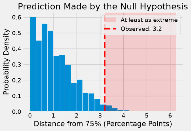
The shaded right tail contains distances at least as large as 3.2 percentage points. Instead of deciding from the position of a dot alone, compute the fraction of simulations in that tail and compare it with the cutoff chosen in advance.
9.3.7. Conventional Cut-offs and the P-value#
A common decision rule uses a significance level of 0.05. Other levels may be appropriate when the costs of false alarms and missed effects differ. The p-value supplies the evidence to which that rule is applied.
The conventions are based on the area in the tail, starting at the observed statistic (the red dashed line) and looking in the direction that makes us lean toward the alternative. In this example that’s the right side, because big distances favor the alternative which says that the model isn’t good.
If the area of the tail is small, the observed statistic is far away from the values most commonly predicted by the null hypothesis.
In this density histogram, area represents probability. To find the area in the tail, we have to find the percent of distances that were greater than or equal to 3.2, where the red dashed line is. The array distances contains the distances for all 10,000 repetitions of random sampling under Mendel’s model, and different_observed_statistic is 3.2.
p_value = np.mean(distances >= different_observed_statistic)
print('Simulated p-value:', round(p_value, 4))
Simulated p-value: 0.0274
The output above estimates the probability of a distance at least as large as 3.2 under Mendel’s model. This is a simulation estimate: another set of random draws will give a slightly different value. More repetitions generally make the estimate more stable.
9.3.7.1. The p-Value#
This chance has an impressive name. It is called the observed significance level of the test. That’s a mouthful, and so it is commonly called the p-value of the test.
Definition: The p-value of a test is the chance, based on the model in the null hypothesis, that the test statistic will be equal to the observed value in the sample or even further in the direction that supports the alternative.
If a p-value is small, that means the tail beyond the observed statistic is small and so the observed statistic is far away from what the null predicts. This implies that the data give evidence against the null hypothesis.
How small is “small”? According to the conventions:
With a significance level of 5%, reject the null if the p-value is below 0.05. This is called a statistically significant result at that level.
A p-value below 1% is sometimes labeled “highly statistically significant.” Report the actual p-value: this label does not measure the size or business value of an effect.
For this simulation, the p-value is below 0.05. So the conventional conclusion would be to reject the null hypothesis and say that the data are not consistent with Mendel’s model for the new plants. Formally, the result of the test is statistically significant.
When you make a conclusion in this way, we recommend that you don’t just say whether or not the result is statistically significant. Along with your conclusion, provide the observed statistic and the p-value as well, so that readers can use their own judgment.
Two ways a test can be wrong. A test makes its decision from random data, so the decision can be wrong in two different ways:
Decision |
The null hypothesis is true |
The null hypothesis is false |
|---|---|---|
Reject the null |
Type I error (a false alarm) |
Correct decision |
Do not reject the null |
Correct decision |
Type II error (a missed effect) |
A Type I error rejects a null hypothesis that is actually true. The cutoff controls how often this happens: if you reject whenever the p-value is below 5%, then a correctly calibrated test has a long-run false-alarm rate at most about 5% when the null is true. Discrete test statistics can make the rate lower. That cutoff is called the significance level of the test.
A Type II error fails to reject a null hypothesis that is actually false. How often this happens depends on how far the truth is from the null hypothesis and on the sample size. Small samples often miss real differences.
For example, an online store tests whether a new checkout page changes the purchase rate. The null hypothesis is that it makes no difference. A Type I error means rolling out a page that doesn’t really help, which wastes development effort. A Type II error means dropping a page that would have increased sales, which is a missed gain. Lowering the cutoff from 5% to 1% makes Type I errors rarer but Type II errors more common, unless the store collects more data.
Read the p-value carefully: It is a probability of results under the null model. It is not the probability that the null is true, and it is not the probability that the result occurred “by chance.” A large p-value means insufficient evidence to reject the model, rather than proof that it is correct.
Statistical and practical importance: Suppose a large checkout experiment estimates a purchase-rate increase from 10.00% to 10.02%, with p = 0.003. At a preselected 5% level, the result is statistically significant. For 100,000 monthly visits, the estimated increase is 20 purchases. At \(10 contribution per purchase, that is \)200 per month. A $1,000 monthly operating cost would exceed the estimated gain. The statistical conclusion alone does not justify rollout. The effect estimate is uncertain too, so report that uncertainty when it is available.
A cutoff on the statistic: For a distance statistic, a 5% upper-tail rule can also be expressed using a high percentile of the null distribution. The pattern np.percentile(simulated_statistics, 95) finds an estimated 95th-percentile boundary. Compare the observed statistic with the unrounded boundary, and round only for display. With a small or discrete simulation, ties and percentile interpolation mean this need not agree exactly with a p-value rule.
# A small illustrative null distribution, sorted here for easy inspection.
import numpy as np
simulated_statistics = np.array([0.01, 0.02, 0.03, 0.04, 0.05,
                                 0.06, 0.07, 0.08, 0.09, 0.10])
observed_distance = 0.098
cutoff_value = np.percentile(simulated_statistics, 95)
print('95th percentile:', round(cutoff_value, 3))
print('Observed is above it:', observed_distance > cutoff_value)
print('Tail fraction:', np.mean(simulated_statistics >= observed_distance))
# The cutoff is 0.0955 before rounding. The tail fraction is 0.1 because
# ten repetitions allow proportions only in steps of 0.1. Use many more
# repetitions for an actual test, especially near a decision boundary.
95th percentile: 0.095
Observed is above it: True
Tail fraction: 0.1
### Exercise: Interpret a Business Result
# A checkout change has p = 0.003 and an estimated purchase-rate gain
# of 0.02 percentage points. Assume 100,000 visits per month,
# $10 contribution per extra purchase, and $1,000 monthly operating cost.
# Compute the estimated extra purchases and net monthly contribution.
# Explain in a comment why statistical significance alone is insufficient.
visits = 100000
increase_percentage_points = 0.02
contribution_per_purchase = 10
monthly_cost = 1000
### Your code starts here.

### Your code ends here.
Estimated extra purchases: 20
Estimated net monthly contribution: -800
9.3.8. Historical Note on the Conventions#
The determination of statistical significance, as defined above, has become standard in statistical analyses in all fields of application. When a convention is so universally followed, it is interesting to examine how it arose.
The method of statistical testing – choosing between hypotheses based on data in random samples – was developed by Sir Ronald Fisher in the early 20th century. Sir Ronald might have set the convention for statistical significance somewhat unwittingly, in the following statement in his 1925 book Statistical Methods for Research Workers. About the 5% level, he wrote, “It is convenient to take this point as a limit in judging whether a deviation is to be considered significant or not.”
What was “convenient” for Sir Ronald became a cutoff that has acquired the status of a universal constant. No matter that Sir Ronald himself made the point that the value was his personal choice from among many: in an article in 1926, he wrote, “If one in twenty does not seem high enough odds, we may, if we prefer it draw the line at one in fifty (the 2 percent point), or one in a hundred (the 1 percent point). Personally, the author prefers to set a low standard of significance at the 5 percent point …”
Fisher knew that “low” is a matter of judgment and has no unique definition. We suggest that you too keep this in mind. Provide your data, make your judgment, and explain why you made it.
Whether you use a conventional cutoff or your own judgment, it is important to keep the following points in mind.
Always provide the observed value of the test statistic and the p-value, so that readers can decide whether or not they think the p-value is small.
Don’t look to defy convention only when the conventionally derived result is not to your liking.
Even if a test concludes that the data don’t support the chance model in the null hypothesis, it typically doesn’t explain why the model doesn’t work. Don’t make causal conclusions without further analysis, unless you are running a randomized controlled trial. We will analyze those in a later section.
9.3.9. Section Practice#
Use this short exercise to check the main workflow from this section.
### Exercise: Practice Hypotheses and p-Value
# A website claims that 25% of visitors click its banner. In a sample of 400 visitors,
# 120 clicked (30%). The test statistic is | sample percent - 25 |.
#   1. Compute the observed statistic.
#   2. Simulate 10,000 samples of 400 visitors under the 25% model and compute the
#      statistic for each: rng.binomial(400, 0.25, size=10000) gives the click counts.
#   3. Compute the p-value and decide at the 5% cutoff.
import numpy as np

rng = np.random.default_rng(7)
clicks = 120
visitors = 400
### Your code starts here


### Your code ends here
Observed statistic: 5.0
P-value: 0.0243
Decision: reject the null