
11.1. Percentiles#
A percentile locates a value in ordered numerical data. A delivery manager might use a high percentile of delivery times to describe a service target; the median describes a central delivery time. These summaries answer different business questions.
With ties or a small dataset, more than one percentile convention is possible. This chapter uses NumPy’s nearest convention for percentile calculations and confidence-interval endpoints. It selects an observed value near a position in the sorted list. A percentile is not a guarantee that exactly the stated fraction lies strictly below it.
For an ordinary median, use np.median(values) or series.median(): with an even number of observations, average the two middle values. A nearest-method 50th percentile can differ from that ordinary median. You will see that distinction below.
Run the demonstration cells in order. Each Interactive Exercise includes independent setup.
11.1.1. Estimation Prelude#
In the previous chapter, we began to develop ways of inferential thinking. In particular, we learned how to use data to decide between two hypotheses about the world. But often we just want to know how big something is.
For example, during an election year, we may want to know the percentage of voters who favor a particular candidate. To assess the current state of the economy, we might be interested in the median annual income of households in the United States.
In this chapter, we will develop a way to estimate an unknown parameter. Remember that a parameter is a numerical value associated with a population.
To figure out the value of a parameter, we need data. If we have the relevant data for the entire population, we can simply calculate the parameter.
However, if the population is very large – for example, if it comprises all the households in the United States – then gathering data from the entire population might be too expensive and time-consuming. In such situations, data scientists rely on random sampling from the population.
This raises a question of inference: How can justifiable conclusions be drawn about the unknown parameter based on the data from the random sample? We will answer this question by using inferential thinking.
A statistic based on a random sample can be a reasonable estimate of an unknown parameter in the population. For example, you might want to use the median annual income of sampled households as an estimate of the median annual income of all households in the U.S.
However, the value of any statistic depends on the sample, which is based on random draws. So every time data scientists come up with an estimate based on a random sample, they are faced with a question:
“How different could this estimate have been, if the sample had come out differently?”
In this chapter, you will learn one way of answering this question. The answer will provide you with the tools to estimate a numerical parameter and quantify the error in your estimate. We will start with a preliminary about percentiles. The most famous percentile is the median, often used in summaries of income data. Other percentiles will be important in the method of estimation that we are about to develop. So we will start by defining percentiles carefully.
For a store, the population might be all completed orders in a specified month, the parameter their mean value, and the estimate the mean of a random sample. Specify the population and measurement period before sampling. An estimate of a monthly mean does not describe every individual order.
The percentile calculations below first summarize observed data. Later, the same calculation selects endpoints from a distribution of bootstrap statistics, rather than from the individual observations.
11.1.2. A Numerical Example#
Consider the following five continent areas, rounded to the nearest million square miles. A percentile calculation first sorts the values. Under the nearest convention, the 80th percentile selects the value nearest position (5 - 1) * 80 / 100 = 3.2, counting the first sorted position as zero. Position three contains 12.
sizes = np.array([12, 17, 6, 9, 7])
Sort the data before interpreting a percentile. The zero-based positions will be zero through four.
np.sort(sizes)
array([ 6, 7, 9, 12, 17])
The sorted values are [6, 7, 9, 12, 17]. The nearest position to 3.2 is three, so the nearest-method 80th percentile is 12. Four of these five values, or 80%, are less than or equal to 12.
For the 70th percentile, the position is (5 - 1) * 70 / 100 = 2.8. Its nearest integer is also three, so the answer is again 12. With a small dataset, different percentile requests can select the same observed value.
11.1.3. The percentile function#
The pattern is np.percentile(values, percentage, method='nearest'). The data come first, followed by a percentage from zero to 100 inclusive. You can pass a list of percentages to request several values at once.
NumPy’s default method is linear, which can interpolate between observations. This chapter explicitly requests nearest to keep the convention visible. Other methods, such as inverted_cdf, implement different rules; they are not interchangeable on small datasets. See the NumPy percentile documentation.
np.percentile(values, percentage, method='nearest')
np.percentile(values, [25, 50, 75], method='nearest')
These are syntax patterns: replace values with your array or Series and percentage with the requested percentage. The next cell applies the pattern to the continent data.
np.percentile(sizes, 70, method='nearest')
np.int64(12)
11.1.3.1. The General Definition#
For this chapter’s nearest convention, sort the n observations and calculate the zero-based position j = (n - 1) * p / 100. Select the observed value at the nearest integer position. At an exact halfway tie, NumPy rounds to the even index. The zero and 100th percentiles select the minimum and maximum, respectively.
You can reproduce this indexing rule with index = int(np.rint(j)), then access sorted_values[index]. np.rint rounds to the nearest integer with the same even-index tie rule.
A different, valid convention uses the one-based rank ceil(n * p / 100) for positive p. That is the inverse empirical-distribution convention, available as method='inverted_cdf'. It is not the nearest rule used here. For the homework order values, the two rules give different first and third quartiles, so always state the method used.
For [1, 2, 3, 4], the nearest-method 50th percentile selects index two, giving 3. The ordinary median averages 2 and 3, giving 2.5. Use the ordinary median consistently when the statistic being bootstrapped is called the sample median.
### Exercise: Compare Two Conventions
# For these four values, compute the nearest-method 50th percentile and
# the ordinary median. Print both and explain their difference in a comment.
import numpy as np
values = np.array([1, 2, 3, 4])
### Your code starts here.

### Your code ends here.
Nearest 50th percentile: 3
Ordinary median: 2.5
11.1.3.2. Example#
The table scores_and_sections contains one row for each student in a class of 359 students. The columns are the student’s discussion section and midterm score.
scores_and_sections = pd.read_csv(path_data + 'scores_by_section.csv')
scores_and_sections
| Section | Midterm | |
|---|---|---|
| 0 | 1 | 22 |
| 1 | 2 | 12 |
| 2 | 2 | 23 |
| 3 | 2 | 14 |
| 4 | 1 | 20 |
| ... | ... | ... |
| 354 | 5 | 24 |
| 355 | 2 | 16 |
| 356 | 2 | 17 |
| 357 | 12 | 16 |
| 358 | 10 | 14 |
359 rows × 2 columns
from matplotlib.ticker import FuncFormatter

fig, ax = plt.subplots(figsize=(5,3))

ax.hist(
    scores_and_sections['Midterm'],
    bins = np.arange(-0.5, 25.6, 1),
    density=True,
    alpha=0.8,
    ec='white')

unit = ''
y_label = 'Percent per ' + (unit if unit else 'unit')
x_label = 'Midterm'

plt.ylabel(y_label)
plt.xlabel(x_label)
y_vals = ax.get_yticks()
# ax.set_yticklabels(['{:g}'.format(x * 100) for x in y_vals])
ax.yaxis.set_major_formatter(FuncFormatter(lambda y, _: '{:.0f}%'.format(y*100)))

plt.title('Distribution of Midterm Scores');
# ax.set_title('Distribution of Midterm Scores')
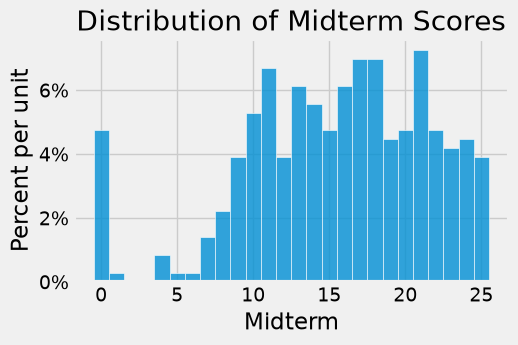
What was the 85th percentile of the scores? To use the percentile function, create an array scores containing the midterm scores, and find the 85th percentile:
scores = scores_and_sections.iloc[:,1]  ### select the second column of the DataFrame,
                                        ### which contains the midterm scores.
scores.head()
0    22
1    12
2    23
3    14
4    20
Name: Midterm, dtype: int64
# np.percentile(scores, 85, method='nearest')  # nearest interpolation method is used to find the 85th percentile of the scores.
np.percentile(scores, 85, method='nearest')  # nearest interpolation method is used to find the 85th percentile of the scores.
np.int64(22)
The nearest-method 85th percentile is 22. Check its selected index directly, rather than assuming that another percentile convention must give the same rank.
First, put the scores in increasing order:
sorted_scores = np.sort(scores_and_sections.iloc[:, 1])
sorted_scores
array([ 0,  0,  0,  0,  0,  0,  0,  0,  0,  0,  0,  0,  0,  0,  0,  0,  0,
        1,  4,  4,  4,  5,  6,  7,  7,  7,  7,  7,  8,  8,  8,  8,  8,  8,
        8,  8,  9,  9,  9,  9,  9,  9,  9,  9,  9,  9,  9,  9,  9,  9, 10,
       10, 10, 10, 10, 10, 10, 10, 10, 10, 10, 10, 10, 10, 10, 10, 10, 10,
       10, 11, 11, 11, 11, 11, 11, 11, 11, 11, 11, 11, 11, 11, 11, 11, 11,
       11, 11, 11, 11, 11, 11, 11, 11, 12, 12, 12, 12, 12, 12, 12, 12, 12,
       12, 12, 12, 12, 12, 13, 13, 13, 13, 13, 13, 13, 13, 13, 13, 13, 13,
       13, 13, 13, 13, 13, 13, 13, 13, 13, 13, 14, 14, 14, 14, 14, 14, 14,
       14, 14, 14, 14, 14, 14, 14, 14, 14, 14, 14, 14, 14, 15, 15, 15, 15,
       15, 15, 15, 15, 15, 15, 15, 15, 15, 15, 15, 15, 15, 16, 16, 16, 16,
       16, 16, 16, 16, 16, 16, 16, 16, 16, 16, 16, 16, 16, 16, 16, 16, 16,
       16, 17, 17, 17, 17, 17, 17, 17, 17, 17, 17, 17, 17, 17, 17, 17, 17,
       17, 17, 17, 17, 17, 17, 17, 17, 17, 18, 18, 18, 18, 18, 18, 18, 18,
       18, 18, 18, 18, 18, 18, 18, 18, 18, 18, 18, 18, 18, 18, 18, 18, 18,
       19, 19, 19, 19, 19, 19, 19, 19, 19, 19, 19, 19, 19, 19, 19, 19, 20,
       20, 20, 20, 20, 20, 20, 20, 20, 20, 20, 20, 20, 20, 20, 20, 20, 21,
       21, 21, 21, 21, 21, 21, 21, 21, 21, 21, 21, 21, 21, 21, 21, 21, 21,
       21, 21, 21, 21, 21, 21, 21, 21, 22, 22, 22, 22, 22, 22, 22, 22, 22,
       22, 22, 22, 22, 22, 22, 22, 22, 23, 23, 23, 23, 23, 23, 23, 23, 23,
       23, 23, 23, 23, 23, 23, 24, 24, 24, 24, 24, 24, 24, 24, 24, 24, 24,
       24, 24, 24, 24, 24, 25, 25, 25, 25, 25, 25, 25, 25, 25, 25, 25, 25,
       25, 25])
There are 359 scores. The nearest-method zero-based position is (359 - 1) * 0.85, or 304.3.
(len(sorted_scores) - 1) * 0.85
304.3
Round 304.3 to index 304, which is the 305th element of the sorted list. The next cell selects that value.
# The 305th sorted value is at zero-based index 304.
sorted_scores[304]
np.int64(22)
That’s the same as the answer we got by using percentile. In future, we will just use percentile.
11.1.4. Quartiles#
The first and third quartiles are the 25th and 75th percentiles. State the convention used when reporting them. Here, calculate them with nearest and calculate the ordinary median separately.
For these 359 scores, the ordinary median and nearest-method 50th percentile agree because the list has an odd length. That agreement is not guaranteed with an even sample size.
q_25 = np.percentile(scores, 25, method='nearest').item()
median = np.median(scores).item()
q_75 = np.percentile(scores, 75, method='nearest').item()
print('25th percentile:', q_25)
print('Median:', median)
print('75th percentile:', q_75)
25th percentile: 11
Median: 16.0
75th percentile: 20
The interval from the first to the third quartile describes the middle of the individual scores. It is not a confidence interval for a population mean or median. With ties and finite-sample percentile conventions, it need not contain exactly 50% of observations.
11.1.5. Section Practice#
Use this short exercise to check the main workflow from this section.
### Exercise: Practice Percentiles
# A call center recorded 12 hold times in minutes.
#   1. Compute the nearest-method 90th percentile.
#   2. Check it by sorting the values and selecting the index nearest
#      (n - 1) * 0.90. Use int(np.rint(...)) for NumPy's tie convention.
#   3. Print both results.
import numpy as np
hold_times = np.array([3, 7, 2, 12, 5, 4, 9, 6, 15, 3, 8, 5])
### Your code starts here.

### Your code ends here.
np.percentile: 12
Definition: 12