
10.3. Causality#
A well-run randomized experiment uses chance to assign participants to treatment and control. That design supports a causal interpretation because assignment does not systematically depend on participants’ pre-existing characteristics. Groups can still differ by chance, which is why you compare the observed difference with a randomization distribution.
A causal conclusion also depends on how the experiment was conducted. Missing outcomes, inconsistent treatment delivery, or one participant’s treatment changing another’s outcome can complicate the interpretation. Random assignment is a design tool, not a guarantee that every source of bias has vanished.
Comparison |
Statistic and direction |
What the design supports |
|---|---|---|
Smoking groups |
Smokers minus nonsmokers; left tail |
Association under the sampling and null-model assumptions. |
Football teams |
Patriots minus Colts; right tail |
A model check for measured pressure drops. |
Randomized trial |
Absolute difference in relief rates; right tail |
Evidence of a treatment effect for study participants under the trial assumptions. |
The same permutation workflow serves all three cases. The study design determines how far you can take the conclusion. Run the demonstration cells in order.
10.3.1. Treating Chronic Back Pain: A Randomized Controlled Trial#
Low-back pain in adults can be very persistent and hard to treat. Common methods run the gamut from corticosteroids to acupuncture. A randomized controlled trial (RCT) examined the effect of using Botulinum Toxin A (BTA) as a treatment. Botulinum toxin is a neurotoxic protein that causes the disease botulism; Wikipedia says that botulinum “is the most acutely lethal toxin known.” There are seven types of botulinum toxin. Botulinum Toxin A is one of the types that can cause disease in humans, but it is also used in medicine to treat various diseases involving the muscles. The RCT analyzed by Foster, Clapp, and Jabbari in 2001 examined it as a treatment for low back pain.
Thirty one patients with low-back pain were randomized into treatment and control groups, with 15 in the treatment group and 16 in control. The control group was given normal saline, and the trials were run double-blind so that neither doctors nor patients knew which group they were in.
Eight weeks after the start of the study, nine of the 15 in the treatment group and two of the 16 in the control group had pain relief (according to a precise definition used by the researchers). These data are in the table bta and appear to show that the treatment has a clear benefit.
bta = pd.read_csv(path_data + 'bta.csv')
bta.tail(10)
| Group | Result | |
|---|---|---|
| 21 | Treatment | 1.0 |
| 22 | Treatment | 1.0 |
| 23 | Treatment | 1.0 |
| 24 | Treatment | 1.0 |
| 25 | Treatment | 0.0 |
| 26 | Treatment | 0.0 |
| 27 | Treatment | 0.0 |
| 28 | Treatment | 0.0 |
| 29 | Treatment | 0.0 |
| 30 | Treatment | 0.0 |
Let’s see how many patients recovered in each group. Remember that counting is the same as adding zeros and ones. The sum of 1’s in the control group is the number of control group patients who had pain relief.
bta_group = bta.groupby('Group').mean()
bta_group.reset_index()
| Group | Result | |
|---|---|---|
| 0 | Control | 0.125 |
| 1 | Treatment | 0.600 |
In the treatment group, 60% of the patients had pain relief, compared to only 12.5% in the control group. None of the patients suffered any side effects.
So the indications are that botulinum toxin A did better than the saline. But the conclusion isn’t yet a slam-dunk. The patients were assigned at random into the two groups, so perhaps the difference could just be due to chance?
To understand what this means, we have to consider the possibility that among the 31 patients in the study, some were simply better able to recover than others, even without any help from the treatment. What if an unusually large proportion of such patients got assigned to the treatment group, just by chance? Then even if the treatment did nothing more than the saline in the control group, the results of the treatment group might look better than those of the control group.
To account for this possibility, let’s start by carefully setting up the chance model.
10.3.2. Potential Outcomes#
Before the patients are randomized into the two groups, our minds instinctively imagine two possible outcomes for each patient: the outcome that the patient would have if assigned to the treatment group, and the outcome that the same patient would have if assigned to the control group. These are called the two potential outcomes of the patient.
Thus there are 31 potential treatment outcomes and 31 potential control outcomes. The question is about the distributions of these two sets of 31 outcomes each. Are they the same, or are they different?
We can’t answer this just yet, because we don’t get to see all 31 values in each group. We just get to see a randomly selected 16 of the potential control outcomes, and the treatment outcomes of the remaining 15 patients.
Here is a good way to visualize the setting. Each patient has a two-sided ticket:
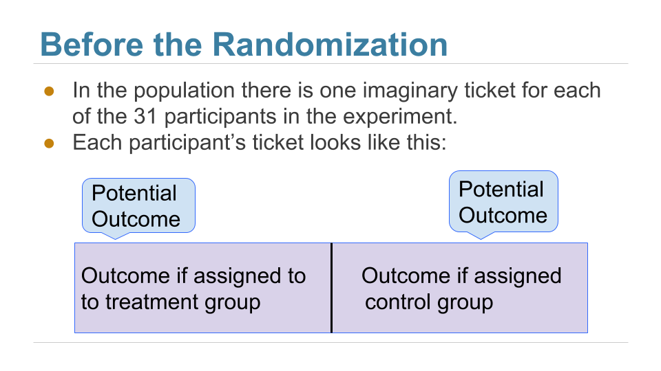
Fig. 10.1 Each patient has a potential outcome under treatment and under control.#
After the randomization, we get to see the right half of a randomly selected set of tickets, and the left half of the remaining group.
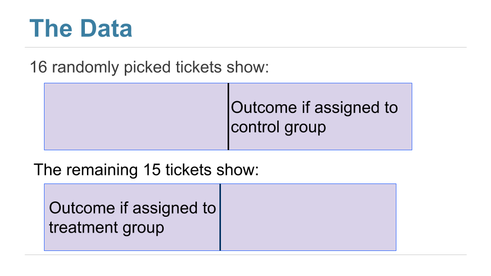
Fig. 10.2 Random assignment reveals one potential outcome per patient; the other stays unknown.#
The table observed_outcomes collects the information about every patient’s potential outcomes, leaving the unobserved half of each “ticket” blank. (It’s just another way of thinking about the bta table, carrying the same information.)
Each patient has two potential outcomes, but the trial reveals only the outcome under the assigned condition. An unobserved outcome is unknown, not a zero. Random assignment lets you compare groups to estimate an average effect; it does not reveal an individual’s missing potential outcome.
### Exercise: Identify the Missing Outcome
# A customer is assigned to checkout B and makes a purchase.
# Can you observe whether that same customer would have purchased under A
# on this occasion? Print observed or unknown and explain in a comment.
### Your code starts here.

### Your code ends here.
unknown
observed_outcomes = pd.read_csv(path_data + "observed_outcomes.csv")
observed_outcomes.head(10)
| Group | Outcome if assigned treatment | Outcome if assigned control | |
|---|---|---|---|
| 0 | Control | Unknown | 1 |
| 1 | Control | Unknown | 1 |
| 2 | Control | Unknown | 0 |
| 3 | Control | Unknown | 0 |
| 4 | Control | Unknown | 0 |
| 5 | Control | Unknown | 0 |
| 6 | Control | Unknown | 0 |
| 7 | Control | Unknown | 0 |
| 8 | Control | Unknown | 0 |
| 9 | Control | Unknown | 0 |
10.3.3. The Hypotheses#
For this randomization test, use a no-effect null hypothesis: each patient’s relief outcome would be the same under treatment and under control. This is called a sharp null because it specifies the missing potential outcome for every patient. Under that null, the observed zeros and ones stay fixed while the random treatment assignment varies.
Null Hypothesis: Treatment has no effect on any patient’s recorded relief outcome. Differences between the randomized groups arise from assignment alone.
Alternative Hypothesis: Treatment affects relief outcomes for some patients. The observed difference in group relief rates can provide evidence against the no-effect null.
Equal overall rates of potential outcomes are a weaker claim than no effect for every patient: benefits for some and harms for others could cancel. The simple shuffle below represents the stronger no-effect model. A test based on a rate difference may not detect effects that cancel in the average.
Use a two-sided statistic because either an increase or a decrease in relief would matter. Choose this direction and the significance level before looking at the result. For a question specifically about improvement, state a one-sided alternative in advance and retain the sign of the treatment-minus-control difference.
Under the sharp null, any random subset of 15 of the 31 patients can receive treatment and the remaining 16 control. Permuting the labels preserves those group sizes and the 31 observed outcomes. That is the same computational pattern used earlier; here, the actual random assignment justifies the reference distribution.
10.3.4. The Test Statistic#
If the two group proportions are very different from each other, we will lean towards the alternative hypothesis that the two underlying distributions are different. So our test statistic will be the distance between the two group proportions, that is, the absolute value of the difference between them.
Large values of the test statistic will favor the alternative hypothesis over the null.
Since the two group proportions were 0.6 and 0.125, the observed value of the test statistic is \(\big{\vert} 0.6 - 0.125 \big{\vert} = 0.475\).
bta_group = bta.groupby('Group').mean()

bta_group = bta_group.reset_index()

bta_group
| Group | Result | |
|---|---|---|
| 0 | Control | 0.125 |
| 1 | Treatment | 0.600 |
observed_proportions = bta_group['Result']
observed_distance = abs(observed_proportions.iloc[0] - observed_proportions.iloc[1])
observed_distance
np.float64(0.475)
As we have done before, we will define a function that takes the following arguments:
the name of the table of data
the column label of the numerical variable
the column label of the group labels
and returns the distance between the two group proportions.
def distance(table, label, group_label):
    reduced = table[[label, group_label]]               ### select cols
    proportions = reduced.groupby(group_label).mean()   ### group means
    distance = proportions[label]                       ### extract means
    return abs(distance.iloc[1] - distance.iloc[0])     ### calc difference
distance(bta_group, 'Result', 'Group')
np.float64(0.475)
10.3.5. Predicting the Statistic Under the Null Hypothesis#
We can simulate results under the null hypothesis, to see how our test statistic should come out if the null hypothesis is true.
10.3.5.1. Generating One Value of the Statistic#
The simulation follows exactly the same process we used in the previous section. We start by randomly permuting the all group labels and then attaching the shuffled labels to the 0/1 results.
### create a copy and shuffle group labels

bta_with_shuffled_labels = bta.copy()                                   ### 1. create a copy to keep bta intact

shuffled_groups = bta['Group'].sample(len(bta), replace=False).values   ### 2. shuffle series => array

bta_with_shuffled_labels['Shuffled Label'] = shuffled_groups            ### 3. add to df
bta_with_shuffled_labels.head()

### notes on shuffling ###
# bta['Group'].sample(len(bta), replace=False)          ### sample returns series, pandas reorder by index
# bta['Group'].sample(len(bta), replace=False).info     ### series
# bta['Group'].sample(len(bta), replace=False).shape    ### 1D
# bta['Group'].sample(len(bta), replace=False).values   ### .values returns np.array
| Group | Result | Shuffled Label | |
|---|---|---|---|
| 0 | Control | 1.0 | Control |
| 1 | Control | 1.0 | Control |
| 2 | Control | 0.0 | Control |
| 3 | Control | 0.0 | Treatment |
| 4 | Control | 0.0 | Control |
Note that numpy does have a permutation() function that would do the same job but it is nice to have a workflow that we can learn and control all the steps.
bta_shuffled = bta.copy()
bta_shuffled['Shuffled Label'] = np.random.permutation(bta['Group'])
bta_shuffled.head()
| Group | Result | Shuffled Label | |
|---|---|---|---|
| 0 | Control | 1.0 | Control |
| 1 | Control | 1.0 | Treatment |
| 2 | Control | 0.0 | Treatment |
| 3 | Control | 0.0 | Control |
| 4 | Control | 0.0 | Control |
We can now find the distance between the two proportions after the group labels have been shuffled.
distance(bta_with_shuffled_labels, 'Result', 'Shuffled Label')
np.float64(0.041666666666666685)
This is quite different from the distance between the two original proportions.
distance(bta_with_shuffled_labels, 'Result', 'Group')
np.float64(0.475)
10.3.5.2. Permutation Test#
If we shuffled the labels again, how different would the new distance be? To answer this, we will define a function that simulates one simulated value of the distance under the hypothesis of random draws from the same underlying distribution. And then we will collect 20,000 such simulated values in an array.
You can see that we are doing exactly what we did in our previous examples of the permutation test.
def one_simulated_distance(table, label, group_label):

    temp_table = table.copy()                                                       ### 1.copy tbl
    shuffled_labels = table[group_label].sample(len(table), replace=False).values   ### 2.shuffle labels
    temp_table['Shuffled Label'] = shuffled_labels                                  ### 3.add series

    shuffled_means = temp_table.groupby('Shuffled Label')[label].mean()             ### 4.means of groups

    return distance(shuffled_means.reset_index(), label, 'Shuffled Label')          ### 5.return distance


### use permutation() to shuffle
# shuffled_labels = np.random.permutation(table[group_label])
np.random.seed(42)
distances = np.array([])
repetitions = 20000
for _ in range(repetitions):
    distances = np.append(distances, one_simulated_distance(bta, 'Result', 'Group'))
### Exercise: Interpret a Two-Sided Distance
# The statistic is the absolute difference in relief proportions.
# Compute the simulated tail fraction, including a result equal to observed.
import numpy as np
observed = 0.3
simulated = np.array([0.0, 0.1, 0.3, 0.4, 0.2])
### Your code starts here.

### Your code ends here.
Tail fraction: 0.4
10.3.6. Conclusion of the Test#
The array distances contains 20,000 values of our test statistic simulated under the null hypothesis. Here is their empirical histogram along with the observed value of the statistic. To find the P-value of the test, remember that large values of the distance favor the alternative hypothesis.
empirical_P = np.mean(distances >= observed_distance)
print('Observed distance:', observed_distance)
print('Simulated p-value:', round(empirical_P, 4))
fig, ax = plt.subplots(figsize=(7, 4))
ax.hist(distances, bins=np.arange(0, 0.85, 0.05), density=True, edgecolor='white')
ax.axvline(observed_distance, color='red', linestyle='--', label='Observed: 0.475')
ax.axvspan(observed_distance, 0.8, color='gold', alpha=0.3,
           label='At least as extreme: right tail')
ax.set_xlabel('Absolute Difference in Relief Proportions')
ax.set_ylabel('Probability Density')
ax.set_title('Prediction Under the No-Effect Null')
ax.legend()
Observed distance: 0.475
Simulated p-value: 0.0092
<matplotlib.legend.Legend at 0x7f6ec6c201a0>
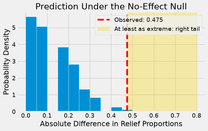
To find the empirical p-value numerically, we must find the proportion of simulated statistics that were equal to or larger than the observed statistic. So the empirical P-value is the proportion of simulated statistics that were equal to or larger than the observed statistic.
empirical_P = np.count_nonzero(distances >= observed_distance) / repetitions
empirical_P
np.float64(0.0092)
This is a small p-value. The observed statistic is in the tail of the empirical histogram of the test statistic generated under the null hypothesis.
The result is statistically significant. The test favors the alternative hypothesis over the null. The evidence supports the hypothesis that the treatment is doing something.
The study reports a P-value of 0.009, or 0.9%, which is not far from our empirical value.
10.3.7. Causality#
The randomized design and small p-value provide evidence of a treatment effect on recorded relief for these study participants, assuming the trial was conducted as described. The observed treatment relief rate is higher, so the estimated direction is beneficial. The absolute-distance p-value alone would not tell you that direction.
Random assignment prevents systematic allocation based on pre-existing patient characteristics; it does not force the two small groups to be identical. The randomization test accounts for differences that assignment alone can produce. Comparable follow-up, consistent outcome measurement, and the absence of interference between patients also matter.
Without random assignment, a similar difference could reflect other characteristics of the groups. For example, people with more severe initial pain might be more likely to seek treatment and might also have different recovery patterns. Such a variable is a confounder when its effects are mixed with the treatment comparison.
Random sampling answers a separate question: to whom can you generalize? A trial of volunteers can support a causal comparison for its participants while leaving uncertainty about other patients or settings.
Sample size and power: Statistical power is the chance of detecting an effect of a specified size with a specified test. A small trial can miss a real effect and gives an imprecise estimate. A larger sample improves precision under otherwise comparable conditions, but cannot repair biased assignment or unequal follow-up. Failure to reject is insufficient evidence of an effect, not proof of no effect.
10.3.8. A Meta-Analysis#
While the RCT does provide evidence that the botulinum toxin A treatment helped patients, a study of 31 patients isn’t enough to establish the effectiveness of a medical treatment. This is not just because of the small sample size. Our results in this section are valid for the 31 patients in the study, but we are really interested in the population of all possible patients.
In 2011, a group of researchers performed a meta-analysis of the studies on the treatment. That is, they identified all the available studies of such treatments for low-back pain and summarized the collated results.
There were several studies but not many could be included in a scientifically sound manner: “We excluded evidence from nineteen studies due to non-randomisation, incomplete or unpublished data.” Only three randomized controlled trials remained, one of which is the one we have studied in this section. The meta-analysis gave it the highest assessment among all the studies (LBP stands for low-back pain): “We identified three studies that investigated the merits of BoNT for LBP, but only one had a low risk of bias and evaluated patients with non-specific LBP (N = 31).”
Putting it all together, the meta-analysis concluded, “There is low quality evidence that BoNT injections improved pain, function, or both better than saline injections and very low quality evidence that they were better than acupuncture or steroid injections. … Further research is very likely to have an important impact on the estimate of effect and our confidence in it. Future trials should standardize patient populations, treatment protocols and comparison groups, enlist more participants and include long-term outcomes, cost-benefit analysis and clinical relevance of findings.”
It takes a lot of careful work to establish that a medical treatment has a beneficial effect. Knowing how to analyze randomized controlled trials is a crucial part of this work. Now that you know how to do that, you are well positioned to help medical and other professions establish cause-and-effect relations.
10.3.9. Section Practice#
Use this short exercise to check the main workflow from this section.
### Exercise: Practice Causality
# A company randomly assigned 80 employees with back pain to a standing-desk program
# (treatment) or to no program (control) and recorded who reported relief.
#   1. Compute the proportion with relief in each group.
#   2. Compute the difference, treatment minus control.
#   3. Because assignment was random, what can the company conclude if a
#      permutation test gives a small p-value?
import pandas as pd

trial = pd.DataFrame({
    'group': ['treatment', 'control'],
    'relief': [17, 6],
    'no_relief': [23, 34],
})
### Your code starts here


### Your code ends here
       group  relief  no_relief  proportion
0  treatment      17         23       0.425
1    control       6         34       0.150
Difference: 0.275