

12.3. Diagnostics and Inference#
A least squares line can be fitted to any scatter plot. The formulas from Regression Line return a slope and an intercept even when the points follow a curve, and the computer does not warn you. A manager who trusts the line without checking may order the wrong amount of stock or promise a budget result that never arrives.
This section asks two questions before you rely on a line. First, is a straight line the right description? Diagnostics answer that, mainly with plots of the residuals. Second, how much could the slope change with a different sample? The bootstrap from Chapter 11 gives a confidence interval for the slope and a test of whether it could be 0.
12.3.1. Residual Plots#
Recall from Regression Line that the residual for an observation is the observed value minus the fitted value:
A positive residual means the line predicted too low; a negative residual means it predicted too high. A residual plot is a scatter plot of the residuals against the feature (or against the fitted values). A horizontal line at 0 marks a perfect prediction.
Start with the 40 stores. The file store_ad_sales.csv is a simulated teaching data set, not real store records. Each row has the weekly ad spend and weekly sales, both in thousands of dollars.
stores = pd.read_csv(path_data + 'store_ad_sales.csv')

store_slope = slope(stores, 'ad_spend', 'sales')
store_intercept = intercept(stores, 'ad_spend', 'sales')

stores['fitted'] = store_slope * stores['ad_spend'] + store_intercept
stores['residual'] = stores['sales'] - stores['fitted']

print('Slope:    ', round(store_slope, 2))
print('Intercept:', round(store_intercept, 2))
stores[['store', 'ad_spend', 'sales', 'fitted', 'residual']].head().round(2)
Slope:     3.87
Intercept: 57.54
| store | ad_spend | sales | fitted | residual | |
|---|---|---|---|---|---|
| 0 | S01 | 6.0 | 77.3 | 80.75 | -3.45 |
| 1 | S02 | 7.2 | 85.3 | 85.39 | -0.09 |
| 2 | S03 | 2.0 | 50.2 | 65.27 | -15.07 |
| 3 | S04 | 3.4 | 69.8 | 70.69 | -0.89 |
| 4 | S05 | 10.0 | 91.4 | 96.23 | -4.83 |
Here is the scatter plot with the line, and next to it the residual plot. Each point on the right is the vertical distance from a point on the left to the line, so the line in the left plot becomes the flat line at 0 in the right plot.
fig, (ax1, ax2) = plt.subplots(1, 2, figsize=(10, 3.8))

ax1.scatter(stores['ad_spend'], stores['sales'], s=20)
xs = np.array([stores['ad_spend'].min(), stores['ad_spend'].max()])
ax1.plot(xs, store_slope * xs + store_intercept, color='gold', lw=3)
ax1.set_xlabel('Weekly ad spend ($1,000s)')
ax1.set_ylabel('Weekly sales ($1,000s)')
ax1.set_title('Sales and the fitted line')

ax2.scatter(stores['ad_spend'], stores['residual'], s=20)
ax2.axhline(0, color='gold', lw=3)
ax2.set_xlabel('Weekly ad spend ($1,000s)')
ax2.set_ylabel('Residual ($1,000s)')
ax2.set_title('Residuals show no pattern')

plt.tight_layout()
plt.show()
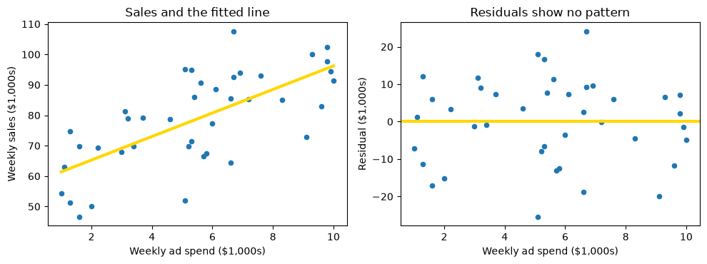
This is what a healthy residual plot looks like. Look for three things:
No pattern. The points form a shapeless cloud. There is no curve, no tilt, and no clump of points on one side of 0 at some range of ad spend.
Centered on 0. In every range of ad spend, the residuals average out near 0. (Equal counts are not the test: many small negative residuals can balance a few large positive ones.)
Even spread. The cloud is about as tall at the left end as at the right end.
When all three hold, the straight line has captured the main trend, and what is left over looks like random noise. In the store data the line is a reasonable model.
The plot is centered on 0 for a reason that is not a coincidence. For the least squares line, the residuals always average to zero. You can check this directly.
print('Average residual:', round(stores['residual'].mean(), 10))
print('Smallest residual:', round(stores['residual'].min(), 2))
print('Largest residual: ', round(stores['residual'].max(), 2))
print('Residual SD:      ', round(stores['residual'].std(ddof=0), 2))
Average residual: 0.0
Smallest residual: -25.37
Largest residual:  24.04
Residual SD:       11.11
The average residual is 0 (to rounding error). This holds for every least squares line, however poor, so the average cannot tell you whether a line is good. That is why you look at the shape of the residual plot, not just its center.
The residual SD of about 11.1 ($11,100) is the typical size of a miss. Individual misses run from about -25 to 24, but they show no pattern.
### Exercise: Residuals of Sales on Staff
#   1. Fit the least squares line of sales on staff (number of employees), using the
#      slope and intercept functions.
#   2. Compute the residuals: sales minus the fitted values.
#   3. Print the average residual, rounded to 6 decimals.
#   4. Print the smallest and largest residuals, rounded to 2 decimals.
# Print exactly:
#   Average residual: <value>
#   Smallest residual: <value>
#   Largest residual: <value>
### Your code starts here.


### Your code ends here.
Average residual: 0.0
Smallest residual: -30.99
Largest residual: 23.76
12.3.2. Detecting Nonlinearity#
Suppose a retailer records, for 104 weeks (the file price_demand.csv is another simulated teaching data set), the price of one product and the number of units sold that week. The prices were changed regularly. In Correlation you saw that price and units are strongly related. What happens when you fit a straight line? Linearity is the assumption that the average outcome changes by a constant amount per unit of the predictor, so that a straight line describes the pattern. A residual plot is the standard check.
pd_data = pd.read_csv(path_data + 'price_demand.csv')

pd_slope = slope(pd_data, 'price', 'units')
pd_intercept = intercept(pd_data, 'price', 'units')
pd_data['fitted'] = pd_slope * pd_data['price'] + pd_intercept
pd_data['residual'] = pd_data['units'] - pd_data['fitted']

print('Correlation:', round(correlation(pd_data, 'price', 'units'), 3))
print('Slope:      ', round(pd_slope, 2))
print('Intercept:  ', round(pd_intercept, 2))
Correlation: -0.951
Slope:       -27.94
Intercept:   458.57
The correlation is about -0.95, which is strong. The slope says that each $1 increase in price goes with about 28 fewer units sold per week. Now look at the scatter plot and at the residuals.
fig, (ax1, ax2) = plt.subplots(1, 2, figsize=(10, 3.8))

ax1.scatter(pd_data['price'], pd_data['units'], s=20)
xs = np.array([pd_data['price'].min(), pd_data['price'].max()])
ax1.plot(xs, pd_slope * xs + pd_intercept, color='gold', lw=3)
ax1.set_xlabel('Price ($)')
ax1.set_ylabel('Units sold per week')
ax1.set_title('The points bend away from the line')

ax2.scatter(pd_data['price'], pd_data['residual'], s=20)
ax2.axhline(0, color='gold', lw=3)
ax2.set_xlabel('Price ($)')
ax2.set_ylabel('Residual (units)')
ax2.set_title('Residuals form a U shape')

plt.tight_layout()
plt.show()
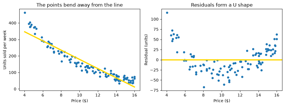
In the left plot the points sag below the line in the middle and rise above it at both ends. The residual plot shows the same thing more clearly: the residuals are positive at low prices, negative at middle prices, and positive again at high prices. This U shape is the signature of a nonlinear relationship. The residuals still average 0, as they must, but they are not random. At a given price, the line is wrong in a predictable direction.
The correlation of -0.95 hid this. A high |r| says the points are close to a line, but the residual plot shows that a curve would do better. You can see the cost by comparing predictions for particular prices with the weeks’ actual sales.
low = pd_data[pd_data['price'] < 6]
mid = pd_data[(pd_data['price'] > 9) & (pd_data['price'] < 12)]
high = pd_data[pd_data['price'] > 14]

print('Average residual, prices under $6:   ', round(low['residual'].mean(), 1), 'units')
print('Average residual, prices $9 to $12:  ', round(mid['residual'].mean(), 1), 'units')
print('Average residual, prices over $14:   ', round(high['residual'].mean(), 1), 'units')
Average residual, prices under $6:    47.3 units
Average residual, prices $9 to $12:   -27.7 units
Average residual, prices over $14:    18.9 units
At prices under $6 the line under-predicts sales by about 47 units a week on average, and at prices over $14 by about 19 units. In the middle of the price range ($9 to $12) it over-predicts by about 28 units. A manager using this line to plan inventory would stock too few units at the lowest prices and too many at mid-range prices.
What can be done when residuals are curved? There are three common responses.
Transform the data. Demand often falls by a constant percentage for each extra dollar of price, not by a constant number of units. Taking the logarithm of units, and keeping price in dollars, turns such a relationship into a straight line. The example below shows this.
Fit a curve. Choose the curve that minimizes the root mean squared error, just as least squares does for the line (Regression Line). Chapter 13 develops this further (Multiple Regression).
Use the line only over a narrow range. Over a short stretch of prices the curve is nearly straight, so a line can serve as a local approximation. It should then not be used outside that range.
Here is the first response. Fit a line to the logarithm of units against price, and draw the residuals.
pd_data['log_units'] = np.log(pd_data['units'])

log_slope = slope(pd_data, 'price', 'log_units')
log_intercept = intercept(pd_data, 'price', 'log_units')
pd_data['log_residual'] = pd_data['log_units'] - (log_slope * pd_data['price'] + log_intercept)

fig, ax = plt.subplots(figsize=(6, 3.8))
ax.scatter(pd_data['price'], pd_data['log_residual'], s=20)
ax.axhline(0, color='gold', lw=3)
ax.set_xlabel('Price ($)')
ax.set_ylabel('Residual (log units)')
ax.set_title('After taking the log of units, the U shape is gone')
plt.show()

print('Slope on the log scale:', round(log_slope, 3))
print('Change in units per extra $1:', round(100 * (np.exp(log_slope) - 1), 1), '%')
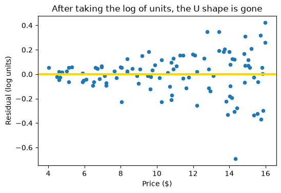
Slope on the log scale: -0.184
Change in units per extra $1: -16.8 %
The residuals no longer curve; they center on 0 across the price range. (They do spread out at high prices, where sales are small: uneven spread, the next topic.) The slope on the log scale is about -0.18: each extra $1 of price goes with about 17% fewer units sold. That is about 34 units where the product sells 200 a week but only about 9 where it sells 50, which is why a straight line in units missed in a U shape.
### Exercise: Curved Residuals in Two Price Ranges
#   1. Using the data below, fit a line of units on price with the slope and
#      intercept functions.
#   2. Compute the residuals: units minus the fitted values.
#   3. Print the average residual for the three cheapest prices and for the
#      three prices in the middle (items 4 to 6), rounded to 1 decimal.
#      Are the two averages on opposite sides of 0, as in a U shape?
# Print exactly:
#   Average residual, cheapest 3: <value>
#   Average residual, middle 3: <value>
ex_demand = pd.DataFrame({
    'price': [4, 5, 6, 8, 10, 12, 14, 15],
    'units': [300, 220, 170, 120, 90, 75, 60, 55],
})
### Your code starts here.


### Your code ends here.
Average residual, cheapest 3: 12.0
Average residual, middle 3: -26.8
12.3.3. Detecting Uneven Spread#
A line can also be wrong in a different way. Even if the trend is straight, the points may be much more spread out in one part of the plot than in another.
Here is a real example. The data are 5,000 yellow-taxi trips in New York City from March 4 to 10, 2019, taken from the 2019 Yellow Taxi Trip Data published by the NYC Taxi and Limousine Commission on NYC Open Data. Each trip has the pickup time, the trip distance in miles, and the metered fare in dollars (before tips, tolls, and surcharges). The extract takes trips spread over every hour of the week, drops trips with zero or negative distance or fare, fares above $150, and trips longer than 40 miles (likely data-entry errors), and keeps a random 5,000. No values were changed. Fit the line of fare on distance.
taxi = pd.read_csv(path_data + 'nyc_taxi_fares.csv')

taxi_slope = slope(taxi, 'distance_miles', 'fare')
taxi_intercept = intercept(taxi, 'distance_miles', 'fare')
taxi['fitted'] = taxi_slope * taxi['distance_miles'] + taxi_intercept
taxi['residual'] = taxi['fare'] - taxi['fitted']

print('Trips:      ', len(taxi))
print('Correlation:', round(correlation(taxi, 'distance_miles', 'fare'), 3))
print('Slope:      ', round(taxi_slope, 2), 'dollars per mile')
print('Intercept:  ', round(taxi_intercept, 2), 'dollars')
Trips:       5000
Correlation: 0.947
Slope:       2.72 dollars per mile
Intercept:   4.84 dollars
The correlation is about 0.95, so the line looks excellent: each extra mile adds about $2.72 to the fare. Now the pictures. With 5,000 points, the plots use small, partly transparent markers so that dense areas look darker.
fig, (ax1, ax2) = plt.subplots(1, 2, figsize=(10, 3.8))

ax1.scatter(taxi['distance_miles'], taxi['fare'], s=6, alpha=0.3)
xs = np.array([0, 40])
ax1.plot(xs, taxi_slope * xs + taxi_intercept, color='gold', lw=3)
ax1.set_xlabel('Trip distance (miles)')
ax1.set_ylabel('Fare ($)')
ax1.set_title('Fares scatter more on long trips')

ax2.scatter(taxi['distance_miles'], taxi['residual'], s=6, alpha=0.3)
ax2.axhline(0, color='gold', lw=3)
ax2.set_xlabel('Trip distance (miles)')
ax2.set_ylabel('Residual ($)')
ax2.set_title('Residuals fan out as distance grows')

plt.tight_layout()
plt.show()
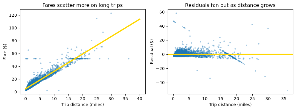
The residuals spread out like a fan: narrow on the left and wide on the right. This is heteroscedasticity (uneven spread); equal spread everywhere is homoscedasticity. A short trip is almost all distance on the meter, while a long trip adds traffic time, route choices, and tolls. The horizontal band at $52 is consistent with the flat fare between Manhattan and JFK, but the data do not record locations, so the extract cannot confirm which $52 fares were JFK trips.
You can measure the change in spread with the residual SD in distance bands.
print('Trips with a recorded fare of $52:', (taxi['fare'] == 52).sum())
print()

short = taxi[taxi['distance_miles'] < 2]
medium = taxi[(taxi['distance_miles'] >= 2) & (taxi['distance_miles'] <= 10)]
long_trips = taxi[taxi['distance_miles'] > 10]

print('Under 2 miles: ', len(short), 'trips, residual SD: $', round(short['residual'].std(ddof=0), 2))
print('2 to 10 miles: ', len(medium), 'trips, residual SD: $', round(medium['residual'].std(ddof=0), 2))
print('Over 10 miles: ', len(long_trips), 'trips, residual SD: $', round(long_trips['residual'].std(ddof=0), 2))
print('All trips:     ', len(taxi), 'trips, residual SD: $', round(taxi['residual'].std(ddof=0), 2))
print()

very_long = taxi[taxi['distance_miles'] > 20]
print('Over 20 miles: ', len(very_long), 'trips, average residual: $', round(very_long['residual'].mean(), 2))
Trips with a recorded fare of $52: 125

Under 2 miles:  2971 trips, residual SD: $ 2.77
2 to 10 miles:  1723 trips, residual SD: $ 3.45
Over 10 miles:  306 trips, residual SD: $ 7.31
All trips:      5000 trips, residual SD: $ 3.52

Over 20 miles:  33 trips, average residual: $ -5.2
The residual SD is about $2.8 for trips under 2 miles and about $7.3 for trips over 10 miles, 2.6 times as large. The overall $3.5 describes neither group well.
The practical consequence is about precision. Up to about 20 miles, the line is a fair guide to the average fare. Beyond 20 miles it over-predicts those 33 trips by about $5 on average, possibly because of flat fares (the data cannot confirm this). And even where the average is right, a prediction for one 15-mile trip can miss by many dollars, while one for a 1-mile trip rarely does. A company forecasting the cost of employee rides should allow a wider margin as distance grows.
### Exercise: Spread by Distance
#   1. Read the taxi data and fit the line of fare on distance with the slope
#      and intercept functions (all 5,000 trips). Compute the residuals.
#   2. Find the residual SD (np.std) for trips of 5 miles or less
#      and for trips over 15 miles, rounded to 2 decimals.
#   3. Print the ratio of the long-trip SD to the short-trip SD, rounded to 1 decimal.
# Print exactly:
#   Up to 5 miles residual SD: <value>
#   Over 15 miles residual SD: <value>
#   Ratio: <value>
### Your code starts here.


### Your code ends here.
Up to 5 miles residual SD: 3.05
Over 15 miles residual SD: 8.22
Ratio: 2.7
12.3.4. Using Diagnostics in Practice#
Before you trust a regression line, run through this short checklist.
Plot the data. Draw the scatter plot. A single number such as r or the slope can look the same for very different pictures.
Plot the residuals. Look for a curve (nonlinearity), a fan (uneven spread), and clumps. A healthy plot is a shapeless cloud centered on 0.
Check the range. A line is a description of the data you have. Use it only for feature values within the range of the data, and avoid extrapolation, which means predicting far outside that range. In the price data, for example, the line would predict negative sales at a price of about $16.40, which is impossible.
Look for influential points. A point far from the others in the feature direction can pull the line toward itself. Refit the line without it. If the slope changes a lot, the line depends on one observation, and you should find out whether that observation is correct.
12.3.4.1. Influential Points#
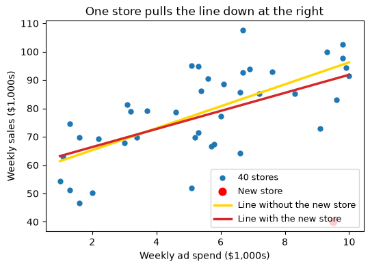
In Correlation you added an invented new store to the 40: it spends $9,500 a week on ads but sells only $40,000, because it has not yet built a customer base. That one store pulled r from about 0.69 down to about 0.54. Here is what it does to the line.
new_store = pd.DataFrame({'store': ['S41'], 'region': ['North'], 'ad_spend': [9.5],
                          'staff': [10], 'store_age': [0], 'sales': [40.0]})
with_new = pd.concat([stores[new_store.columns], new_store], ignore_index=True)

xs = np.array([1, 10])
fig, ax = plt.subplots(figsize=(6, 4))
ax.scatter(stores['ad_spend'], stores['sales'], s=25, label='40 stores')
ax.scatter([9.5], [40.0], s=60, color='red', label='New store')
for data, color, label in [(stores, 'gold', 'Line without the new store'),
                           (with_new, 'tab:red', 'Line with the new store')]:
    ax.plot(xs, slope(data, 'ad_spend', 'sales') * xs + intercept(data, 'ad_spend', 'sales'),
            color=color, lw=2.5, label=label)
ax.set_xlabel('Weekly ad spend ($1,000s)')
ax.set_ylabel('Weekly sales ($1,000s)')
ax.set_title('One store pulls the line down at the right')
ax.legend(fontsize=9)
plt.show()

print('Slope without the new store:', round(slope(stores, 'ad_spend', 'sales'), 2))
print('Slope with the new store:   ', round(slope(with_new, 'ad_spend', 'sales'), 2))
Slope without the new store: 3.87
Slope with the new store:    3.19
One store out of 41 lowers the slope from about 3.87 to about 3.19, a drop of almost a fifth in the estimated sales per $1,000 of ads. The store sits near the right edge of the ad-spend range, far below the line, so it tilts the whole line toward itself. A manager deciding whether ads pay for themselves would read the two slopes very differently. The lesson is the one in the checklist: refit without the point, report both lines, and find out whether the store is typical of the stores the decision is about.
12.3.4.2. Anscombe’s Quartet Revisited#
The quartet from Correlation shows all four checks at once. The four data sets share nearly the same r and the same least squares line. Their residual plots, in the bottom row, tell them apart.
quartet = pd.read_csv(path_data + 'anscombe_quartet.csv')

fig, axes = plt.subplots(2, 4, figsize=(11, 5), sharex=True)
for k, name in enumerate(['I', 'II', 'III', 'IV']):
    part = quartet[quartet['dataset'] == name].copy()
    a_slope = slope(part, 'x', 'y')
    a_intercept = intercept(part, 'x', 'y')
    part['residual'] = part['y'] - (a_slope * part['x'] + a_intercept)
    xs = np.array([3, 20])

    axes[0, k].scatter(part['x'], part['y'], s=25)
    axes[0, k].plot(xs, a_slope * xs + a_intercept, color='gold', lw=3)
    axes[0, k].set_title('Dataset ' + name)
    axes[0, k].set_xlabel('x')

    axes[1, k].scatter(part['x'], part['residual'], s=25)
    axes[1, k].axhline(0, color='gold', lw=3)
    axes[1, k].set_xlabel('x')
    if k == 0:
        axes[0, k].set_ylabel('y')
        axes[1, k].set_ylabel('Residual')

    print('Dataset', name, ' slope:', round(a_slope, 2), ' intercept:', round(a_intercept, 2),
          ' r:', round(correlation(part, 'x', 'y'), 2))

plt.tight_layout()
plt.show()
Dataset I slope: 0.5 intercept: 3.0 r: 0.82
Dataset II  slope: 0.5  intercept: 3.0  r: 0.82
Dataset III  slope: 0.5  intercept: 3.0  r: 0.82
Dataset IV  slope: 0.5  intercept: 3.0  r: 0.82
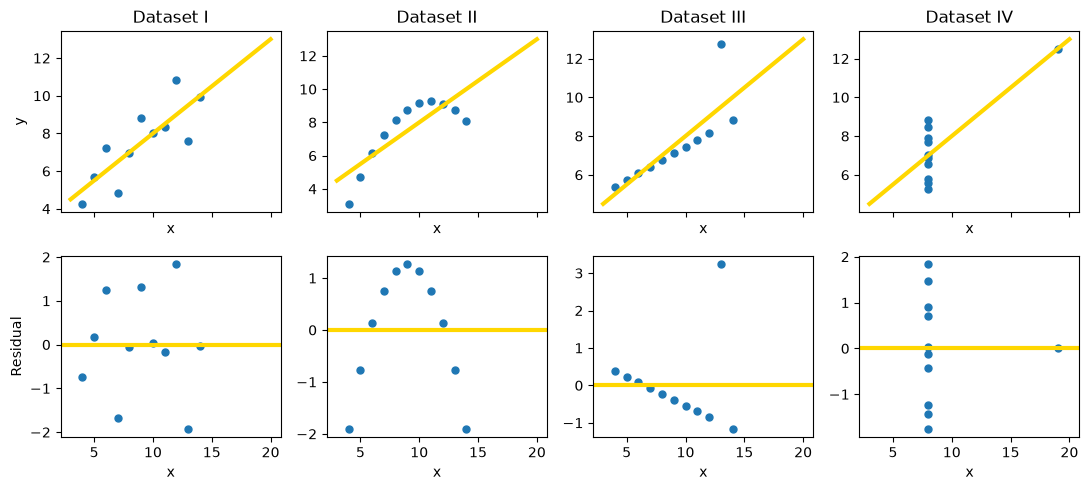
The four lines are essentially the same, but the residual plots tell four different stories: I is a healthy, shapeless cloud; II curves, so the relationship is nonlinear; III is a straight line with one outlier that shows up as one huge residual; and in IV a single point far to the right determines the slope by itself, an influential point. Summary numbers cannot tell these data sets apart. Pictures can.
When a check fails, you do not give up on the data. You transform the variables, fit a curve, restrict the range, or report that the predictions are less precise in some region. The checks also show what is still unsettled. A healthy diagnostic does not prove that a line is the true relationship, and it does not show that one variable causes the other (Comparing Groups Without Random Assignment).
12.3.5. Inference for the Slope#
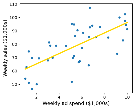
The store data passed the shape checks. Now the manager wants to know whether advertising pays off, and the slope of about 3.87 says that in these 40 stores each extra $1,000 of weekly ad spend goes with about $3,870 more in weekly sales. But the 40 stores are a sample. Imagine the line from all stores like these, observed under conditions like this month’s. Its slope is the true slope, an unknown population parameter, and the sample slope estimates it, as a sample median estimated a population median in The Bootstrap.
observed_slope = slope(stores, 'ad_spend', 'sales')
observed_intercept = intercept(stores, 'ad_spend', 'sales')

fig, ax = plt.subplots(figsize=(5, 4))
ax.scatter(stores['ad_spend'], stores['sales'], s=20)
xs = np.array([1, 10])
ax.plot(xs, observed_slope * xs + observed_intercept, color='gold', lw=3)
ax.set_xlabel('Weekly ad spend ($1,000s)', fontsize=12)
ax.set_ylabel('Weekly sales ($1,000s)', fontsize=12)
plt.show()

print('Slope:    ', round(observed_slope, 2))
print('Intercept:', round(observed_intercept, 2))
Slope:     3.87
Intercept: 57.54
To see that the estimate depends on which stores happen to be in the sample, split the 40 stores into two groups of 20 and fit a line to each.
first_20 = stores.iloc[:20]
last_20 = stores.iloc[20:]

print('Slope from the first 20 stores:', round(slope(first_20, 'ad_spend', 'sales'), 2))
print('Slope from the last 20 stores: ', round(slope(last_20, 'ad_spend', 'sales'), 2))
Slope from the first 20 stores: 5.04
Slope from the last 20 stores:  3.39
The two halves give slopes of about 5.04 and 3.39. Neither is wrong; each is a fair estimate from a smaller sample. A fitted slope has sampling variability, and a manager who reads only one slope does not know whether the true slope might be 3, 4, or 5.
12.3.5.1. Bootstrapping the Slope#
You cannot go back and collect many new samples of stores. As in The Bootstrap, resample the sample: draw 40 rows from stores at random with replacement, and fit a line to the resample. The slope of that line is a bootstrap slope.
One detail matters for regression: resample whole rows. Each row keeps a store’s ad spend and sales together, so the resample keeps the relationship between the two variables. Resampling the two columns separately would break every pair and destroy the association you want to measure.
def one_bootstrap_slope():
    resample = stores.sample(len(stores), replace=True)
    return slope(resample, 'ad_spend', 'sales')
Run the cell below a few times. Each run gives a slightly different slope.
one_bootstrap_slope().item()
4.239651875636567
Now repeat the process 5,000 times and collect the slopes, as you collected medians and means in Chapter 11.
# Seed once so the example is reproducible; do not reset inside the loop.
np.random.seed(42)

num_repetitions = 5000
bstrap_slopes = np.array([])
for i in np.arange(num_repetitions):
    bstrap_slopes = np.append(bstrap_slopes, one_bootstrap_slope())

len(bstrap_slopes)
5000
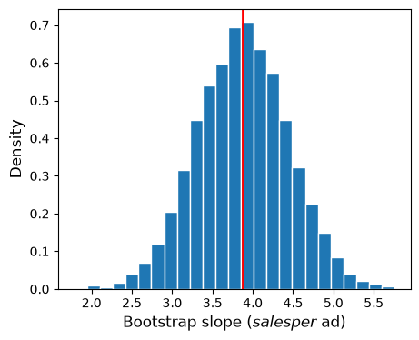
The 5,000 bootstrap slopes form the empirical distribution of the slope. The histogram shows how much the slope moves from resample to resample; the red line marks the slope of the original sample.
fig, ax = plt.subplots(figsize=(5, 4))
ax.hist(bstrap_slopes, bins=25, density=True, ec='white')
ax.axvline(observed_slope, color='red', lw=2)
ax.set_xlabel('Bootstrap slope ($ sales per $ ad)', fontsize=12)
ax.set_ylabel('Density', fontsize=12)
plt.show()
### Exercise: Bootstrap the Staffing Slope
# Does sales rise with the number of staff?
#   1. Write a function that resamples the rows of stores with replacement,
#      using stores.sample(len(stores), replace=True, random_state=seed),
#      and returns the slope of sales on staff.
#   2. Collect 1,000 bootstrap slopes with seed = 0, 1, ..., 999.
#   3. Print the observed slope, the number of bootstrap slopes, and the smallest
#      and largest bootstrap slopes, rounded to 2 decimals.
### Your code starts here.


### Your code ends here.
Observed slope: 1.95
Number of bootstrap slopes: 1000
Smallest and largest: -0.04 3.98
12.3.5.2. A Confidence Interval and a Test#
The bootstrap percentile method from Confidence Intervals works for slopes exactly as it did for medians and means. For a 95% confidence interval, take the 2.5th and 97.5th percentiles of the bootstrap slopes.
left = np.percentile(bstrap_slopes, 2.5, method='nearest')
right = np.percentile(bstrap_slopes, 97.5, method='nearest')

np.array([left, right]).round(2)
array([2.79, 4.98])
fig, ax = plt.subplots(figsize=(5, 4))
ax.hist(bstrap_slopes, bins=25, density=True, ec='white')
ax.plot([left, right], [0, 0], color='yellow', lw=8)
ax.set_xlabel('Bootstrap slope ($ sales per $ ad)', fontsize=12)
ax.set_ylabel('Density', fontsize=12)
plt.show()
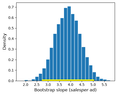
The approximate 95% confidence interval for the true slope runs from about 2.79 to 4.98.
Business interpretation. Across the chain’s stores, each extra $1,000 of weekly ad spend is associated with between about $2,790 and $4,980 more in weekly sales, at 95% confidence. As in Chapter 11, the 95% describes the method: intervals built this way would contain the true slope about 95% of the time.
The interval describes an association: stores that spend more on ads may also differ in location or size (Correlation). That matters for the manager’s real question. Suppose each dollar of sales brings 30 cents of gross profit. Then advertising pays for itself only if one extra dollar of ads causes more than \(1/0.30 \approx 3.33\) dollars of sales. An interval for an association cannot answer that causal question, and even if the slope were causal, the interval reaches below 3.33. To decide, the manager needs evidence about cause, such as an experiment that randomly assigns ad budgets to stores (Causality).
A slope of 0 means the best-fitting straight line is flat: \(x\) has no linear association with \(y\) (the average of \(y\) could still change along a curve, as in the profit example of Correlation). In the language of Hypotheses and p-Values:
Null hypothesis: the true slope is 0; the sample slope differs from 0 only by chance.
Alternative hypothesis: the true slope is not 0.
If 0 is outside the 95% confidence interval, reject the null hypothesis at about the 5% cutoff (the bootstrap interval is approximate, so the test is too). If 0 is inside, the data are consistent with no linear association. For ad spend, 0 is far outside 2.79 to 4.98, so you reject the null hypothesis.
Now a different question: do older stores sell more? Here is the slope of sales on store_age.
age_slope = slope(stores, 'store_age', 'sales')
round(age_slope.item(), 2)
-0.28
In the sample, each extra year open goes with about $280 less in weekly sales. Is that a real pattern, or chance? Bootstrap the slope and check whether 0 is in the interval.
def one_bootstrap_age_slope():
    resample = stores.sample(len(stores), replace=True)
    return slope(resample, 'store_age', 'sales')

np.random.seed(42)
age_slopes = np.array([])
for i in np.arange(5000):
    age_slopes = np.append(age_slopes, one_bootstrap_age_slope())

age_left = np.percentile(age_slopes, 2.5, method='nearest')
age_right = np.percentile(age_slopes, 97.5, method='nearest')
np.array([age_left, age_right]).round(2)
array([-0.97, 0.37])
fig, ax = plt.subplots(figsize=(5, 4))
ax.hist(age_slopes, bins=25, density=True, ec='white')
ax.plot([age_left, age_right], [0, 0], color='yellow', lw=8)
ax.axvline(0, color='red', lw=2)
ax.set_xlabel('Bootstrap slope (sales on store age)', fontsize=12)
ax.set_ylabel('Density', fontsize=12)
plt.show()
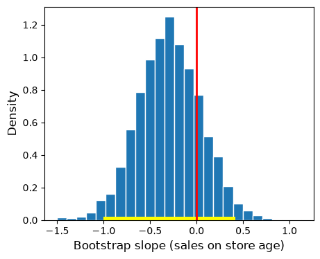
The interval runs from about -0.97 to 0.37 and contains 0 (the red line), so you do not reject the null hypothesis: the manager should not conclude that older stores sell less. Not rejecting is not proving, though. The interval also includes slopes such as -0.8, a loss of $800 a week per year open, and 40 stores cannot rule that out.
### Exercise: Is Staffing Associated with Sales?
#   1. Collect 1,000 bootstrap slopes of sales on staff, using
#      stores.sample(len(stores), replace=True, random_state=i) for i = 0, ..., 999.
#   2. Compute the 95% confidence interval with np.percentile(..., method='nearest').
#   3. Print the interval rounded to 2 decimals and whether 0 is inside it.
# Print exactly:
#   95% interval: 0.86 to 3.05
#   0 inside the interval: False
### Your code starts here.


### Your code ends here.
95% interval: 0.86 to 3.05
0 inside the interval: False
12.3.5.3. Cautions#
The bootstrap interval is only as good as the sample and the line.
Shape and influential points. Run the diagnostics first. If the residuals curve, the slope summarizes the wrong shape; if one store pulls the line, the interval reflects that store more than the chain. A fan does not spoil the interval for the slope, but it makes predictions for single stores less certain in parts of the range.
How the data were collected. The bootstrap assumes the rows are independent draws that represent the population (Confidence Intervals). Resampling these 40 stores mimics drawing other stores under this month’s conditions, not other months, and no plot can check this.
Range and sample size. The interval applies to ad spend between about $1,000 and $10,000 a week. With only a handful of rows, the interval can mislead, and more bootstrap repetitions do not help; only more data does.
12.3.6. Section Practice#
### Exercise: Practice Visual Diagnostics
# A delivery company fits a regression line of delivery cost on distance.
#   1. Fit the line (slope and intercept from r and the SDs) and compute the residuals.
#   2. Draw a residual plot: distance on the x-axis, residual on the y-axis, with a
#      horizontal line at 0.
#   3. Describe the pattern: is it curved, or does the spread change?
# Print exactly:
#   Residuals: [<the 10 residuals, rounded to 1 decimal, as a NumPy array>]
import numpy as np
import matplotlib.pyplot as plt

distance = np.array([2, 4, 6, 8, 10, 12, 14, 16, 18, 20])
cost = np.array([9, 11, 12, 16, 15, 22, 18, 30, 21, 36])
### Your code starts here.


### Your code ends here.
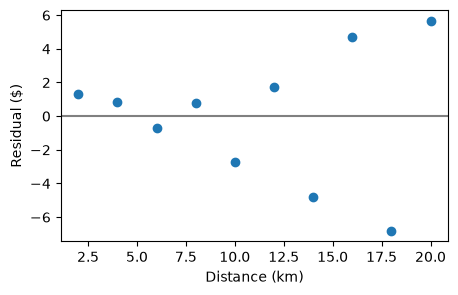
Residuals: [ 1.3 0.8 -0.7 0.8 -2.7 1.7 -4.8 4.7 -6.8 5.7]