Choosing Features and Avoiding Overfitting

13.3. Choosing Features and Avoiding Overfitting#

A real estate analyst at a brokerage wants a model that prices homes before they are listed. In Multiple Regression you saw that adding predictors can help: a home’s price depends on more than its size. That raises an obvious question. If three predictors are better than one, why not use thirty, or all the data the county records?

This section shows why “more is better” is the wrong rule. You will see that a model’s error on the data it was fitted to always falls as features are added, but its error on new homes can rise. You will learn to spot this problem, called overfitting, to choose among models fairly with a validation set, and to weigh accuracy against how easily a model can be explained.

The data are the same Ames, Iowa home sales used in Regression with scikit-learn: real sales from 2006 to 2010, recorded by the Ames Assessor’s Office and published by Dean De Cock in the Journal of Statistics Education (2011). The file keeps normal sales only (foreclosures, family sales, and similar are removed) and drops the few homes over 4,000 square feet that De Cock recommends removing. That leaves 2,412 homes. Prices are in dollars; we report errors in thousands of dollars.

homes = pd.read_csv(path_data + 'ames_housing.csv')
print(len(homes), 'homes')
homes.head()

2412 homes

	sale_price	living_area	overall_quality	year_built	garage_cars	total_rooms	full_baths	lot_area	neighborhood	year_sold
0	215000	1656	6	1960	2	7	1	31770	NAmes	2010
1	105000	896	5	1961	1	5	1	11622	NAmes	2010
2	172000	1329	6	1958	1	6	1	14267	NAmes	2010
3	244000	2110	7	1968	2	8	2	11160	NAmes	2010
4	189900	1629	5	1997	2	6	2	13830	Gilbert	2010

13.3.1. More Features, Better Fit?#

Imagine the analyst has records of only 100 sales to build the model. We take a random sample of 100 homes as the training set, the data used to fit a model, and set the other 2,412 - 100 = 2,312 homes aside. They play no role until the next section.

train_rows, other_rows = train_test_split(homes.index, train_size=100, random_state=1)
train = homes.loc[train_rows]
print('Training homes:', len(train))
print('Set aside for later:', len(other_rows))

Training homes: 100
Set aside for later: 2312

The first column is the most useful predictor: living area. We add the others one at a time, in the order of how an analyst might rank them (size, then quality, then age, then the amenities), refit the model each time, and record the training RMSE, the root mean squared error on the same homes used to fit the model. (RMSE was defined in Regression with scikit-learn.)

numeric = ['living_area', 'overall_quality', 'year_built', 'garage_cars',
           'full_baths', 'lot_area', 'total_rooms']

results = []
for k in range(1, len(numeric) + 1):
    chosen = numeric[:k]
    model = LinearRegression().fit(train[chosen], train['sale_price'])
    train_rmse = rmse(train['sale_price'], model.predict(train[chosen]))
    results.append([k, chosen[-1], round(train_rmse / 1000, 1)])

pd.DataFrame(results, columns=['features', 'last feature added', 'training RMSE ($1,000s)'])

	features	last feature added	training RMSE ($1,000s)
0	1	living_area	44.5
1	2	overall_quality	36.8
2	3	year_built	32.8
3	4	garage_cars	32.0
4	5	full_baths	31.1
5	6	lot_area	24.5
6	7	total_rooms	24.4

Each added feature lowers the training RMSE, from about $44,500 with living area alone to about $24,400 with all seven. This is not a coincidence. Least squares picks the coefficients that make the squared errors on the training data as small as possible. A model with an extra feature can always set that feature’s coefficient to zero and reproduce the smaller model, so the best it can do is the same or better. Training error never rises when a feature is added.

That is true even when the feature is useless. To see this, we add columns of pure random noise: numbers drawn from a normal distribution that have nothing to do with the sales.

rng = np.random.default_rng(0)
noise = pd.DataFrame(rng.normal(size=(len(homes), 10)),
                     columns=['noise' + str(i) for i in range(1, 11)],
                     index=homes.index)

for j in [0, 2, 5, 10]:
    chosen = numeric + list(noise.columns[:j])
    X_train = pd.concat([train[numeric], noise.loc[train_rows]], axis=1)[chosen]
    model = LinearRegression().fit(X_train, train['sale_price'])
    print(j, 'noise columns: training RMSE =',
          round(rmse(train['sale_price'], model.predict(X_train)) / 1000, 2), '($1,000s)')

noise columns: training RMSE = 24.39 ($1,000s)
noise columns: training RMSE = 24.06 ($1,000s)
noise columns: training RMSE = 23.56 ($1,000s)
noise columns: training RMSE = 20.64 ($1,000s)

Ten columns of random numbers lower the training RMSE from $24,390 to $20,640. The model “found” patterns in the noise because with only 100 homes, some combination of random columns always lines up a little with the prices. A manager who judged the model by its training error would conclude that the noise columns are valuable. They are not, and the next section shows how to see that.

Key idea

Training error rewards every feature, useful or not. It cannot tell you which features to keep.

13.3.2. Overfitting #

What we want to know is how well the model prices homes it has not seen. The 2,312 homes we set aside are the test set: they were not used to fit the model, so the RMSE on them estimates how the model will do on new listings (see Regression with scikit-learn for the train/test idea).

We also let the model become much more flexible. Beyond the seven numeric features, we add:

one column for each of the 28 neighborhoods (1 if the home is in that neighborhood, 0 otherwise),
the square of each numeric feature, which lets the model bend,
the product of each pair of numeric features, which lets the effect of one feature depend on another (an interaction).

All numeric features are standardized first (as in Correlation) so squares and products are on a comparable scale.

# Standardize the numeric columns so squares and products are on one scale
Z = (homes[numeric] - homes[numeric].mean()) / homes[numeric].std()

neighborhoods = pd.get_dummies(homes['neighborhood']).astype(float)
squares = pd.DataFrame({a + '^2': Z[a] ** 2 for a in numeric})
products = pd.DataFrame({a + ' x ' + b: Z[a] * Z[b] for a, b in combinations(numeric, 2)})

X_all = pd.concat([Z, neighborhoods, squares, products], axis=1)
n_numeric, n_nbhd, n_sq = len(numeric), neighborhoods.shape[1], squares.shape[1]

print('numeric columns:     ', n_numeric)
print('neighborhood columns:', n_nbhd)
print('squared columns:     ', n_sq)
print('product columns:     ', products.shape[1])
print('all columns:         ', X_all.shape[1])

numeric columns:      7
neighborhood columns: 28
squared columns:      7
product columns:      21
all columns:          63

The columns are ordered from the simplest to the most flexible, so using the first $k$ columns gives a sequence of larger and larger models. For each, we fit on the 100 training homes and compute the RMSE on the training homes and on the test set.

sizes = [1, 2, 3, 4, 5, 6, 7,
         n_numeric + n_nbhd,
         n_numeric + n_nbhd + n_sq,
         X_all.shape[1]]

test_rows = other_rows
curve = []
for k in sizes:
    cols = list(X_all.columns[:k])
    model = LinearRegression().fit(X_all.loc[train_rows, cols], homes.loc[train_rows, 'sale_price'])
    tr = rmse(homes.loc[train_rows, 'sale_price'], model.predict(X_all.loc[train_rows, cols]))
    te = rmse(homes.loc[test_rows, 'sale_price'], model.predict(X_all.loc[test_rows, cols]))
    curve.append([k, round(tr / 1000, 1), round(te / 1000, 1)])

curve = pd.DataFrame(curve, columns=['columns', 'training RMSE', 'test RMSE'])
curve

	columns	training RMSE	test RMSE
0	1	44.5	48.1
1	2	36.8	35.4
2	3	32.8	34.0
3	4	32.0	33.3
4	5	31.1	33.0
5	6	24.5	35.0
6	7	24.4	34.8
7	35	18.7	35.8
8	42	15.6	147.0
9	63	12.6	181.6

Training RMSE falls at every step, from about $44,500 to about $12,600. Test RMSE tells a different story. It falls while the first few features are added, reaches its lowest value of about $33,000 with 5 columns, and then rises: $35,000 at 6 columns, and far worse for the most flexible models, about $147,000 at 42 columns and $182,000 at 63. The 63-column model fits 100 homes with 63 coefficients and a constant, so it chases the quirks of those particular homes. When it prices other homes, its typical error is as large as the average price of a home (about $175,000).

fig, ax = plt.subplots(figsize=(7, 4))
ax.plot(curve['columns'], curve['training RMSE'], marker='o', color='tab:blue', label='Training RMSE')
ax.plot(curve['columns'], curve['test RMSE'], marker='o', color='tab:red', label='Test RMSE')
ax.set_xscale('log')
ax.set_yscale('log')
ax.set_xticks(curve['columns'])
ax.set_xticklabels(curve['columns'])
ax.set_yticks([10, 20, 50, 100, 200])
ax.set_yticklabels([10, 20, 50, 100, 200])
ax.minorticks_off()
ax.set_xlabel('Number of columns in the model (log scale)', fontsize=12)
ax.set_ylabel('RMSE ($1,000s, log scale)', fontsize=12)
ax.set_title('Training error keeps falling; test error turns upward', fontsize=13)
ax.legend()
plt.show()

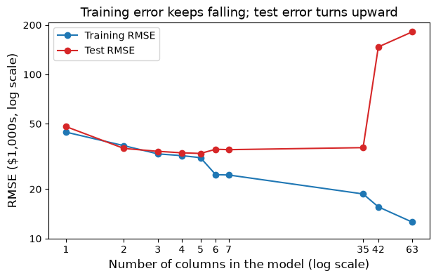
../../_images/ac451d0008349e2ca522a0852bbaf2fd962bf196d49f34df21e3e7619d071cb9.png

This pattern is overfitting: a model fits its training data closely, including its random quirks, and so predicts new data worse. The gap between the two curves is the warning sign. A model whose training error is far below its test error has learned the sample, not the market.

best = curve.loc[curve['test RMSE'].idxmin()]
print('Lowest test RMSE:', best['test RMSE'], 'with', int(best['columns']), 'columns')
print('At', int(curve['columns'].iloc[-1]), 'columns: training RMSE', curve['training RMSE'].iloc[-1],
      'and test RMSE', curve['test RMSE'].iloc[-1])

Lowest test RMSE: 33.0 with 5 columns
At 63 columns: training RMSE 12.6 and test RMSE 181.6

The lesson is not that big models are always bad. The more training data you have compared with the number of columns, the more complexity a model can support. With 100 homes, five or so columns is the limit; with thousands of homes, as in Multiple Regression, seven numeric features are no problem. The right amount of complexity depends on how much data you have.

### Exercise: The Training Gap
#   1. Load ames_housing.csv. Split homes.index with train_test_split(train_size=100, random_state=2); the other rows are the test set.
#   2. Define two feature lists: simple = living_area and overall_quality; full = all seven numeric features, in this order: living_area, overall_quality, year_built, garage_cars, full_baths, lot_area, total_rooms.
#   3. For each list, fit LinearRegression on the training rows and compute the training RMSE and the test RMSE in $1,000s, rounded to 1 decimal.
#   4. Print both RMSEs for each model and the gap (test minus training). In a comment, say which model looks more overfit.
# Print exactly:
# simple train 36.6 test 35.1 gap -1.4
# full train 28.1 test 33.4 gap 5.3
path_data = '../../data/'
import numpy as np
import pandas as pd
from sklearn.linear_model import LinearRegression
from sklearn.model_selection import train_test_split


### Your code starts here.




### Your code ends here.

simple train 36.6 test 35.1 gap -1.4
full train 28.1 test 33.4 gap 5.3

13.3.3. Validation #

We used the test set above to show overfitting. But suppose you used it to choose a model: try ten models, pick the one with the lowest test RMSE, and report that number. The number is now too optimistic, for the same reason as before. You picked the winner because it did well on those particular homes, so those homes are no longer an honest test. The test set is meant to be used once, at the end.

The fix is a third group of homes. We split the data three ways:

the training set fits each candidate model,
the validation set compares the candidates and chooses one,
the test set is touched once, to report the chosen model’s error.

Here is a split with 150 homes for training, 150 for validation, and the remaining homes for testing.

train_rows3, rest = train_test_split(homes.index, train_size=150, random_state=7)
valid_rows, test_rows3 = train_test_split(rest, train_size=150, random_state=7)

print('Training:  ', len(train_rows3))
print('Validation:', len(valid_rows))
print('Test:      ', len(test_rows3))

Training:   150
Validation: 150
Test:       2112

We fit six candidate models on the training set and compare their RMSE on the validation set.

candidates = [1, 2, 4, 7, n_numeric + n_nbhd, X_all.shape[1]]
y = homes['sale_price']

rows = []
for k in candidates:
    cols = list(X_all.columns[:k])
    model = LinearRegression().fit(X_all.loc[train_rows3, cols], y[train_rows3])
    rows.append([k,
                 round(rmse(y[train_rows3], model.predict(X_all.loc[train_rows3, cols])) / 1000, 1),
                 round(rmse(y[valid_rows], model.predict(X_all.loc[valid_rows, cols])) / 1000, 1)])

val_table = pd.DataFrame(rows, columns=['columns', 'training RMSE', 'validation RMSE'])
val_table

	columns	training RMSE	validation RMSE
0	1	43.6	50.0
1	2	32.7	35.7
2	4	30.1	35.7
3	7	26.9	33.5
4	35	22.3	32.8
5	63	13.8	36.1

The training RMSE falls steadily from $43,600 to $13,800 as columns are added, while the validation RMSE is lowest, about $32,800, for the 35-column model (the seven numeric features plus neighborhood). The 63-column model has the lowest training error but a validation RMSE of $36,100, a sign of overfitting. We choose the 35-column model and only now use the test set.

best_k = int(val_table.loc[val_table['validation RMSE'].idxmin(), 'columns'])
cols = list(X_all.columns[:best_k])
final = LinearRegression().fit(X_all.loc[train_rows3, cols], y[train_rows3])
test_rmse = rmse(y[test_rows3], final.predict(X_all.loc[test_rows3, cols]))

print('Chosen by validation RMSE:', best_k, 'columns')
print('Test RMSE, reported once: ', round(test_rmse / 1000, 1), '($1,000s)')

Chosen by validation RMSE: 35 columns
Test RMSE, reported once:  31.5 ($1,000s)

The analyst can tell the broker that the chosen model should price new homes with a typical error of about $31,500. Because the test set played no part in choosing, that is an honest estimate.

Rule

Fit on the training set. Choose on the validation set. Report once on the test set.

13.3.3.1. Cross-Validation #

With 300 homes, a validation set of 150 is a noisy judge: a different random split might choose a different model. Cross-validation uses the data more efficiently. In 5-fold cross-validation, the labeled homes are divided into 5 equal groups (folds). Each fold takes a turn as the validation set while the model is fitted on the other four, and the five RMSEs are averaged. scikit-learn does the whole loop in one call, cross_val_score. We apply it to the 300 homes used for training and validation, still keeping the test set out of sight.

pool = list(train_rows3) + list(valid_rows)   # the 300 homes used for choosing

for k in candidates:
    cols = list(X_all.columns[:k])
    scores = cross_val_score(LinearRegression(), X_all.loc[pool, cols], y[pool],
                             cv=5, scoring='neg_root_mean_squared_error')
    print(k, 'columns: 5-fold RMSE =', round(-scores.mean() / 1000, 1), '($1,000s)')

columns: 5-fold RMSE = 46.9 ($1,000s)
columns: 5-fold RMSE = 34.4 ($1,000s)
columns: 5-fold RMSE = 33.1 ($1,000s)
columns: 5-fold RMSE = 31.2 ($1,000s)
columns: 5-fold RMSE = 29.8 ($1,000s)

63 columns: 5-fold RMSE = 32.2 ($1,000s)

Cross-validation agrees with the validation set about the main point: the 35-column model is best (about $29,800), and the 63-column model is worse (about $32,200). Because every home is used for validation once, the comparison is less affected by the luck of one split. The cost is that the model is fitted five times for each candidate.

### Exercise: Choose by Validation
#   1. Load ames_housing.csv. Split homes.index into 150 training rows and 150 validation rows: first train_test_split(train_size=150, random_state=3) gives training rows and the rest; then split the rest with train_test_split(train_size=150, random_state=3) into validation rows and test rows.
#   2. Candidate models use the first 1, 2, 4, and 7 numeric features, in this order: living_area, overall_quality, year_built, garage_cars, full_baths, lot_area, total_rooms.
#   3. Fit each candidate on the training rows. Compute the validation RMSE in $1,000s, rounded to 1 decimal, and print it for each.
#   4. Print the number of features of the candidate with the lowest validation RMSE, then its test RMSE (rounded to 1 decimal) once.
# Print exactly:
# 1 features: validation RMSE 56.9
# 2 features: validation RMSE 41.5
# 4 features: validation RMSE 37.7
# 7 features: validation RMSE 35.4
# Chosen: 7 features
# Test RMSE: 32.2
path_data = '../../data/'
import numpy as np
import pandas as pd
from sklearn.linear_model import LinearRegression
from sklearn.model_selection import train_test_split


### Your code starts here.




### Your code ends here.

 features: validation RMSE 56.9
2 features: validation RMSE 41.5
4 features: validation RMSE 37.7
7 features: validation RMSE 35.4
Chosen: 7 features
Test RMSE: 32.2

13.3.4. Interpretability #

Accuracy is not the only thing a business needs from a model. A model that a manager can explain is one the manager can check, trust, and defend. A model’s interpretability is how easily people can understand why it gives the predictions it does.

Compare two models for the broker, both fitted on the 300 homes used for training and validation and judged on the test set. One uses three features: living area, overall quality, and year built. The other is the 35-column model, with the seven numeric features and 28 neighborhood indicators.

small = ['living_area', 'overall_quality', 'year_built']
big = list(X_all.columns[:n_numeric + n_nbhd])

simple_model = LinearRegression().fit(homes.loc[pool, small], y[pool])
big_model = LinearRegression().fit(X_all.loc[pool, big], y[pool])

simple_test = rmse(y[test_rows3], simple_model.predict(homes.loc[test_rows3, small]))
big_test = rmse(y[test_rows3], big_model.predict(X_all.loc[test_rows3, big]))

print('3-feature model: test RMSE', round(simple_test / 1000, 1), '($1,000s)')
print('35-column model: test RMSE', round(big_test / 1000, 1), '($1,000s)')

3-feature model: test RMSE 33.0 ($1,000s)
35-column model: test RMSE 30.5 ($1,000s)

The larger model is more accurate on the test set, with an RMSE of about $30,500 against $33,000: a gain of about $2,500 on homes that sell for about $175,000 on average, or roughly 1.4 percent. Is that worth having 35 coefficients instead of three?

It depends on the use. If an automated tool prices thousands of listings and only accuracy matters, the larger model may win. If agents need to explain a price to a seller, the three-feature model has a real advantage, because its whole logic fits in one sentence. Here are its coefficients.

for name, value in zip(small, simple_model.coef_):
    print(f'{name:16s} {value:10.1f}')
print('intercept       ', round(simple_model.intercept_))

living_area            64.9
overall_quality     24275.8
year_built            397.6
intercept        -851224

An agent can say: “Each extra square foot adds about $65, each step of overall quality adds about $24,300, and each year of newer construction adds about $400, other things held fixed.” Each statement can be checked against what the agent sees in the home. Reading 35 coefficients in the same way would be much harder.

13.3.4.1. Report the Uncertainty #

A coefficient from 300 homes is an estimate, so it comes with sampling variability, just like the slope in Inference for the Slope. We use the same remedy: bootstrap the homes, refit the model each time, and take the middle 95 percent of the coefficients.

boot_rng = np.random.default_rng(13)
pool_homes = homes.loc[pool]
boot_coefs = []
for i in range(1000):
    resample = pool_homes.sample(len(pool_homes), replace=True, random_state=boot_rng.integers(1_000_000))
    boot_model = LinearRegression().fit(resample[small], resample['sale_price'])
    boot_coefs.append(boot_model.coef_)
boot_coefs = np.array(boot_coefs)

low, high = np.percentile(boot_coefs, [2.5, 97.5], axis=0)
interval_table = pd.DataFrame({'estimate': simple_model.coef_.round(1),
                               '95% low': low.round(1),
                               '95% high': high.round(1)}, index=small)
interval_table

	estimate	95% low	95% high
living_area	64.9	54.5	75.2
overall_quality	24275.8	19412.9	28990.8
year_built	397.6	229.6	568.9

The interval for living area is about $54 to $75 per square foot, and for year built about $230 to $570 per year. A report that says only “$65 per square foot” suggests more precision than the data support. Giving the interval lets the manager see which coefficients are well pinned down and which are not.

These intervals assume the model is a reasonable description of the data and the homes are like a random sample of the market, the same cautions as in Inference for the Slope. They also describe association: in these records, bigger and better homes sell for more, not that adding a square foot to a particular home would add $65.

13.3.5. Section Practice #

Four models for the brokerage were fitted on a training set and then scored on a validation set and a test set. The RMSEs are in thousands of dollars. Model A uses 3 features, model B uses 5, model C uses 7 features plus neighborhood, and model D adds all squares and interactions (63 columns).

Model	Training RMSE	Validation RMSE	Test RMSE
A (3 features)	34.0	35.2	35.6
B (5 features)	30.5	31.0	31.9
C (35 columns)	22.0	31.8	33.5
D (63 columns)	9.0	48.0	52.0

Which model would you recommend? Model D has by far the lowest training RMSE, but a validation RMSE of 48.0 and a test RMSE of 52.0 show it has overfit. Model C also has a large gap between training and validation. The choice should rest on the validation column: B has the lowest validation RMSE (31.0), so B is chosen, and its test RMSE (31.9) is the number to report. B is also simpler than C, which makes it easier to explain.

### Exercise: Choose a Model
#   1. Build a table (DataFrame) with columns train, valid, and test, with one row per model A, B, C, D, using the RMSEs in the table above (in $1,000s).
#   2. Find the model with the lowest validation RMSE and print its name.
#   3. Print that model's test RMSE.
#   4. Compute each model's gap (validation minus training) and print the model with the largest gap.
# Print exactly:
# Chosen model: B
# Test RMSE: 31.9
# Largest gap: D
path_data = '../../data/'
import numpy as np
import pandas as pd
from sklearn.linear_model import LinearRegression
from sklearn.model_selection import train_test_split


### Your code starts here.




### Your code ends here.

Chosen model: B
Test RMSE: 31.9
Largest gap: D

Choosing Features and Avoiding Overfitting

Contents

13.3. Choosing Features and Avoiding Overfitting#

13.3.1. More Features, Better Fit?#

13.3.2. Overfitting#

13.3.3. Validation#

13.3.3.1. Cross-Validation#

13.3.4. Interpretability#

13.3.4.1. Report the Uncertainty#

13.3.5. Section Practice#