

15.1. Nearest Neighbors with scikit-learn#
In Chapter 14 you built a \(k\)-nearest neighbor classifier by hand (Nearest Neighbors): compute distances, sort, take the \(k\) closest rows, and hold a majority vote. That code shows exactly what the method does, but it is slow and easy to get wrong. In practice, analysts use a library. In Chapter 13 you used scikit-learn’s LinearRegression and KNeighborsRegressor; scikit-learn’s KNeighborsClassifier does the same work for classification, with the same fit and predict steps.
This section follows one business case through the whole workflow, using the online shopping sessions from Sections Classification to Training, Testing, and Accuracy. An online retailer wants to know which sessions are likely to end in a purchase, so that it can send a nudge, such as a reminder email or a free-shipping offer, to those visitors before they leave. The steps are the ones you already know from the hand-built classifier:
Choose the features and the target.
Split the data into a training set and a test set.
Put the features on a common scale, using the training set only.
Fit the classifier, predict, and measure accuracy on the test set.
Choose \(k\) by comparing accuracy on data the classifier has not seen.
15.1.1. The Shopping Session Data#
The file online_shoppers.csv is the real data set introduced in Section Classification: 12,330 sessions on an online retailer’s website over one year, from the UCI Machine Learning Repository (Sakar and others, 2019; CC BY 4.0). Each row is one session. This section uses three numeric attributes and the label:
page_value: the average dollar value of the pages the visitor saw, computed by the retailer’s analytics tool from the sales that followed visits to those pages,exit_rate: how often visits to the pages the visitor saw ended there,product_pages: the number of product pages the visitor viewed,outcome:purchaseif the session ended in a purchase,no purchaseotherwise.
shoppers = pd.read_csv(path_data + 'online_shoppers.csv')

# scikit-learn works with numbers, so make a 0/1 label: 1 means the session ended in a purchase.
shoppers['purchase'] = (shoppers['outcome'] == 'purchase').astype(int)
shoppers[['page_value', 'exit_rate', 'product_pages', 'outcome', 'purchase']].head()
| page_value | exit_rate | product_pages | outcome | purchase | |
|---|---|---|---|---|---|
| 0 | 0.0 | 0.20 | 1 | no purchase | 0 |
| 1 | 0.0 | 0.10 | 2 | no purchase | 0 |
| 2 | 0.0 | 0.20 | 1 | no purchase | 0 |
| 3 | 0.0 | 0.14 | 2 | no purchase | 0 |
| 4 | 0.0 | 0.05 | 10 | no purchase | 0 |
How common is a purchase? The value_counts method with normalize=True gives the proportion of sessions in each class.
shoppers['purchase'].value_counts(normalize=True)
purchase
0    0.845255
1    0.154745
Name: proportion, dtype: float64
About 15% of the sessions ended in a purchase and 85% did not. The classes are imbalanced: one class is much more common than the other. Keep that 85% in mind. A “classifier” that predicts “no purchase” for every session, without looking at any data, is already right about 85% of the time, so a real classifier has to beat that.
Comparing the average attributes of the two groups shows why the features should help.
shoppers.groupby('purchase')[['page_value', 'exit_rate', 'product_pages']].mean()
| page_value | exit_rate | product_pages | |
|---|---|---|---|
| purchase | |||
| 0 | 1.975998 | 0.047378 | 28.714642 |
| 1 | 27.264518 | 0.019555 | 48.210168 |
Sessions that ended in a purchase had an average page value of about $27, compared with about $2 for sessions that did not. Their exit rate was less than half as high (0.020 against 0.047), and they viewed more product pages (48 against 29 on average). These are the same patterns you saw in Section Classification.
### Exercise: Purchase Rate by Visitor Type
#   1. Split the shoppers table into new visitors (visitor_type 'New_Visitor') and
#      returning visitors (visitor_type 'Returning_Visitor').
#   2. Compute the purchase rate (the share of sessions with outcome 'purchase') for
#      each group, rounded to 3 decimals.
# Print exactly:
# Purchase rate, new visitors: 0.249
# Purchase rate, returning visitors: 0.139
ex_visitors = pd.read_csv(path_data + 'online_shoppers.csv')
### Your code starts here.


### Your code ends here.
Purchase rate, new visitors: 0.249
Purchase rate, returning visitors: 0.139
15.1.2. Features, Target, and a Train-Test Split#
As in Chapter 13, scikit-learn expects the inputs in two pieces:
X, a table of features (one column per attribute the classifier may use), andy, the target: the column of labels to predict.
The other columns, such as month and weekend, are not numbers on a common footing with these three, so they are left out to keep the example simple.
features = ['page_value', 'exit_rate', 'product_pages']

X = shoppers[features]
y = shoppers['purchase']

X.shape, y.shape
((12330, 3), (12330,))
Next, hold out a test set. Section Training, Testing, and Accuracy did this by shuffling the rows and cutting the table in two; train_test_split does both steps at once. Keep 30% of the sessions for testing and fix random_state so the split is the same every time the page runs.
The argument stratify=y asks for a stratified split: the training and test sets keep the same share of purchases as the full data. With imbalanced classes this matters, because an unlucky random split could leave the test set with too few purchases to judge the classifier.
X_train, X_test, y_train, y_test = train_test_split(
    X, y, test_size=0.3, random_state=14, stratify=y)

print(len(X_train), 'training sessions and', len(X_test), 'test sessions')
print('Purchase rate in training set:', round(y_train.mean(), 3))
print('Purchase rate in test set:', round(y_test.mean(), 3))
8631 training sessions and 3699 test sessions
Purchase rate in training set: 0.155
Purchase rate in test set: 0.155
Both sets have a purchase rate of about 0.155, the same as the full data. From here on, the test set stays locked away until you are ready to report how well the final classifier works.
### Exercise: A Different Split
#   1. Split X and y again, this time keeping 20% for testing.
#      Use random_state=1 and stratify=y.
#   2. Print the number of training and test sessions and the purchase rate of the
#      test set, rounded to 3 decimals.
# Print exactly:
# Training: 9864
# Test: 2466
# Test purchase rate: 0.155
### Your code starts here.


### Your code ends here.
Training: 9864
Test: 2466
Test purchase rate: 0.155
15.1.3. Scaling Features with StandardScaler#
Distance adds up the squared differences in every feature. The features have very different scales: page value runs from $0 to about $360, the exit rate from 0 to 0.2, and the number of product pages from 0 to 705. Without scaling, a difference of one product page counts as much as a difference of one dollar of page value, even though page value is the strongest sign of a purchase and the number of pages is spread over a far wider range.
In Sections Nearest Neighbors and Training, Testing, and Accuracy you converted each feature to standard units by subtracting its mean and dividing by its SD. scikit-learn’s StandardScaler does the same thing. It works in two steps:
fitlearns the mean and SD of each feature. Fit on the training set only, for the reason given in Section Training, Testing, and Accuracy: the test sessions stand in for future sessions, so they must not influence how the classifier is built.transformapplies those training means and SDs to any table: the training set, the test set, or a brand-new session.
scaler = StandardScaler()
scaler.fit(X_train)

pd.DataFrame({'mean': scaler.mean_, 'SD': scaler.scale_}, index=features)
| mean | SD | |
|---|---|---|
| page_value | 5.818068 | 18.931328 |
| exit_rate | 0.043343 | 0.048874 |
| product_pages | 31.541768 | 44.043043 |
X_train_scaled = scaler.transform(X_train)
X_test_scaled = scaler.transform(X_test)

X_train_scaled[:5].round(2)
array([[-0.31, -0.26, -0.19],
       [ 0.18, -0.64,  4.39],
       [-0.31,  0.07, -0.49],
       [-0.28, -0.59,  4.76],
       [ 0.06, -0.61,  6.39]])
The result is a NumPy array in standard units. Each column of the scaled training set now has mean 0 and SD 1. The scaled test set has means and SDs close to, but not exactly, 0 and 1, because it was scaled with the training statistics, which is what you want.
print('Training means:', X_train_scaled.mean(axis=0).round(2) + 0)
print('Training SDs:  ', X_train_scaled.std(axis=0).round(2))
print('Test means:    ', X_test_scaled.mean(axis=0).round(2))
print('Test SDs:      ', X_test_scaled.std(axis=0).round(2))
Training means: [0. 0. 0.]
Training SDs:   [1. 1. 1.]
Test means:     [ 0.01 -0.02  0.01]
Test SDs:       [0.93 0.98 1.03]
A new session is scaled the same way. Here is a session in which the visitor has viewed 30 product pages, the pages seen have a page value of $12, and the exit rate is 0.02.
new_session = pd.DataFrame({'page_value': [12.0],
                            'exit_rate': [0.02],
                            'product_pages': [30]})

scaler.transform(new_session).round(2)
array([[ 0.33, -0.48, -0.04]])
In standard units, this session’s page value is a third of an SD above average, its exit rate is about half an SD below average, and its number of product pages is almost exactly average.
### Exercise: Scale a New Session
#   1. Put a session with page_value 0.0, exit_rate 0.1, and product_pages 10
#      in a one-row DataFrame with the columns in features.
#   2. Use the scaler fitted above (do not refit it) to convert the session to
#      standard units, and print the result rounded to 2 decimals.
# Print exactly:
# [[-0.31  1.16 -0.49]]
### Your code starts here.


### Your code ends here.
[[-0.31 1.16 -0.49]]
15.1.4. Fitting and Predicting with KNeighborsClassifier#
KNeighborsClassifier is scikit-learn’s \(k\)-nearest neighbor classifier. The argument n_neighbors is \(k\). Fitting a nearest neighbor classifier does very little work: fit simply stores the training rows and their labels. The real work happens in predict, which, for each new row, finds the \(k\) nearest training rows and takes a majority vote, exactly like the classify function you wrote in Section Nearest Neighbors.
knn = KNeighborsClassifier(n_neighbors=5)
knn.fit(X_train_scaled, y_train)
KNeighborsClassifier()In a Jupyter environment, please rerun this cell to show the HTML representation or trust the notebook.
On GitHub, the HTML representation is unable to render, please try loading this page with nbviewer.org.
Parameters
Fitted attributes
To classify the new session from the previous subsection, scale it with the same scaler and call predict.
new_scaled = scaler.transform(new_session)
knn.predict(new_scaled)
array([1])
The prediction is 1: this session is likely to end in a purchase. The kneighbors method shows the evidence behind the vote, the distances to the 5 nearest training sessions and their positions in the training set. Three of the five neighbors ended in a purchase, so the vote is 3 to 2. Looking up those sessions confirms that it is the same distance-and-vote procedure written by hand.
distances, positions = knn.kneighbors(new_scaled)

neighbors = X_train.iloc[positions[0]].copy()
neighbors['purchase'] = y_train.iloc[positions[0]].values
neighbors['distance'] = distances[0].round(3)
neighbors
| page_value | exit_rate | product_pages | purchase | distance | |
|---|---|---|---|---|---|
| 5665 | 12.905876 | 0.018286 | 30 | 0 | 0.059 |
| 4670 | 11.284275 | 0.021453 | 28 | 0 | 0.066 |
| 7428 | 12.587222 | 0.016667 | 28 | 1 | 0.088 |
| 10133 | 13.490319 | 0.019670 | 32 | 1 | 0.091 |
| 10013 | 10.388944 | 0.022857 | 30 | 1 | 0.103 |
Now classify every test session at once and compare the predictions with the actual labels. Accuracy is the proportion of matches; accuracy_score computes it, and so does the classifier’s own score method.
y_pred = knn.predict(X_test_scaled)

print('First ten predictions:', y_pred[:10])
print('First ten actual:     ', y_test.values[:10])
print('Test accuracy:', round(accuracy_score(y_test, y_pred), 3))
First ten predictions: [0 0 0 1 0 0 0 0 0 1]
First ten actual:      [0 0 0 1 0 0 0 0 0 0]
Test accuracy: 0.878
The 5-nearest neighbor classifier is right for 88% of the test sessions, a few points above the 85% of the always-“no purchase” rule.
How much did scaling help? Fit the same classifier on the raw features and compare.
knn_raw = KNeighborsClassifier(n_neighbors=5)
knn_raw.fit(X_train, y_train)

print('Test accuracy without scaling:', round(knn_raw.score(X_test, y_test), 3))
print('Test accuracy with scaling:   ', round(knn.score(X_test_scaled, y_test), 3))
Test accuracy without scaling: 0.876
Test accuracy with scaling:    0.878
Here scaling barely changes the accuracy (0.876 without it, 0.878 with it). That is not because scaling is unimportant. Without scaling, the distance is decided almost entirely by the product page count and the page value, because the exit rate never differs by more than 0.2 and so adds almost nothing. Those two attributes happen to carry most of the signal in this data set, so the accuracy hardly moves. With other attributes, the unscaled classifier could ignore the most useful one, as the product-duration example in Section Nearest Neighbors showed, so scaling is part of the nearest neighbor method, not an optional extra.
### Exercise: Try k = 7
#   1. Fit a KNeighborsClassifier with n_neighbors=7 on X_train_scaled and y_train.
#   2. Predict the test set (X_test_scaled) and print the test accuracy rounded to 3 decimals.
#   3. Predict new_session (use new_scaled) and print the predicted label.
# Print exactly:
# Test accuracy: 0.881
# New session prediction: 0
### Your code starts here.


### Your code ends here.
Test accuracy: 0.881
New session prediction: 0
15.1.5. Pipelines and Choosing k#
Keeping track of a separate scaler and classifier is easy to get wrong, for example by forgetting to scale a new session. A pipeline joins the steps into one object. When you call fit on the pipeline, it fits the scaler on the training data, transforms them, and fits the classifier; when you call predict, it transforms the new rows with the training statistics and then predicts. Scaling with training statistics only is built in.
model = make_pipeline(StandardScaler(), KNeighborsClassifier(n_neighbors=5))
model.fit(X_train, y_train)

print('Test accuracy:', round(model.score(X_test, y_test), 3))
print('New session prediction:', model.predict(new_session)[0])
Test accuracy: 0.878
New session prediction: 1
The pipeline gives the same accuracy and prediction as the two separate steps, and it takes the raw features directly.
Choosing \(k\). The number of neighbors is a choice you make, not something fit learns from the data; such choices are called hyperparameters. A natural idea is to try several values of \(k\) and keep the one with the best test accuracy. But then the test set has been used to build the classifier, and its accuracy is no longer an honest estimate for new sessions, the same problem as testing on the training set, only milder.
The fix is the one from Section Training, Testing, and Accuracy: a validation set. Split the training set once more, use one part to fit and the other part to compare values of \(k\), and save the test set for a single final check. There you sliced the first part of the shuffled training set by hand; train_test_split does it in one call.
X_fit, X_val, y_fit, y_val = train_test_split(
    X_train, y_train, test_size=0.25, random_state=14, stratify=y_train)

print(len(X_fit), 'sessions for fitting and', len(X_val), 'for validation')
6473 sessions for fitting and 2158 for validation
k_values = np.arange(1, 32, 2)     # odd values of k avoid ties in a two-class vote
val_accuracy = []

for k in k_values:
    candidate = make_pipeline(StandardScaler(), KNeighborsClassifier(n_neighbors=k))
    candidate.fit(X_fit, y_fit)
    val_accuracy.append(candidate.score(X_val, y_val))

k_results = pd.DataFrame({'k': k_values, 'validation accuracy': np.round(val_accuracy, 3)})
k_results
| k | validation accuracy | |
|---|---|---|
| 0 | 1 | 0.857 |
| 1 | 3 | 0.886 |
| 2 | 5 | 0.896 |
| 3 | 7 | 0.897 |
| 4 | 9 | 0.897 |
| 5 | 11 | 0.899 |
| 6 | 13 | 0.897 |
| 7 | 15 | 0.897 |
| 8 | 17 | 0.895 |
| 9 | 19 | 0.896 |
| 10 | 21 | 0.896 |
| 11 | 23 | 0.892 |
| 12 | 25 | 0.895 |
| 13 | 27 | 0.893 |
| 14 | 29 | 0.892 |
| 15 | 31 | 0.896 |
fig, ax = plt.subplots(figsize=(6, 3.5))
ax.plot(k_results['k'], k_results['validation accuracy'], marker='o', lw=2)
ax.set_xlabel('k (number of neighbors)')
ax.set_ylabel('Validation accuracy')
plt.show()
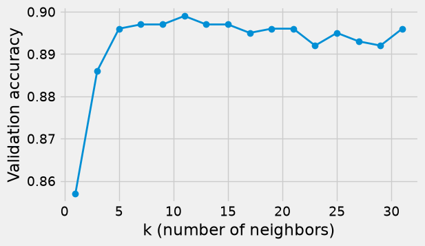
With \(k = 1\) the classifier follows individual training sessions too closely (it overfits), and validation accuracy is lowest. Accuracy rises as \(k\) grows and then levels off at about 0.90; very large \(k\) would eventually blur the pattern, because distant sessions get a vote. Pick the \(k\) with the highest validation accuracy, refit on the whole training set, and check the test set once. Section Training, Testing, and Accuracy compared only \(k\) = 1, 5, 15, and 51 on a different validation set and took 51. Once accuracy levels off, the differences among larger values of \(k\) are small, so a different split or a different list of candidates can pick a different \(k\) with about the same accuracy.
best_k = int(k_results.loc[k_results['validation accuracy'].idxmax(), 'k'])

final_model = make_pipeline(StandardScaler(), KNeighborsClassifier(n_neighbors=best_k))
final_model.fit(X_train, y_train)

print('Chosen k:', best_k)
print('Test accuracy:', round(final_model.score(X_test, y_test), 3))
Chosen k: 11
Test accuracy: 0.888
Validation accuracy is highest at \(k = 11\) (0.899), but every \(k\) from 5 to 31 is within about one percentage point of it. Differences that small are partly the luck of which sessions landed in the validation set, so any \(k\) in that range is a reasonable choice. With \(k = 11\), the final classifier is right for about 89% of the test sessions, compared with 85% for the always-“no purchase” baseline.
### Exercise: Compare a Few Values of k
#   1. For k in [3, 7, 15], fit a pipeline (StandardScaler, then
#      KNeighborsClassifier) on X_fit, y_fit and compute its accuracy on X_val, y_val.
#   2. Print each k with its validation accuracy rounded to 3 decimals, then
#      print the k with the highest validation accuracy.
# Print exactly:
# k = 3 validation accuracy: 0.886
# k = 7 validation accuracy: 0.897
# k = 15 validation accuracy: 0.897
# Best k: 7
### Your code starts here.


### Your code ends here.
k = 3 validation accuracy: 0.886
k = 7 validation accuracy: 0.897
k = 15 validation accuracy: 0.897
Best k: 7