

15.3. Logistic Regression#
A nearest neighbor classifier answers “purchase” or “no purchase”. For many business decisions, a probability is more useful: a session with a 90% chance of ending in a purchase deserves a nudge right now, one with a 15% chance might get a cheaper one, and one with a 1% chance can be left alone. Section Evaluating Classifiers also suggested that when a missed buyer costs much more than a false alarm, it may pay to flag sessions whose chance of a purchase is below 50%. That requires a classifier that reports how likely each outcome is.
Logistic regression is the most widely used classifier of this kind. Despite its name, it is a classification method: it predicts the probability that an observation belongs to the positive class. It builds on the linear regression of Chapter 13, so its coefficients can be read in a similar way. This section fits it to the same real shopping session data (UCI Online Shoppers Purchasing Intention, Sakar and others, 2019; CC BY 4.0), training set, and test set as Sections Nearest Neighbors with scikit-learn and Evaluating Classifiers.
15.3.1. The Logistic Curve#
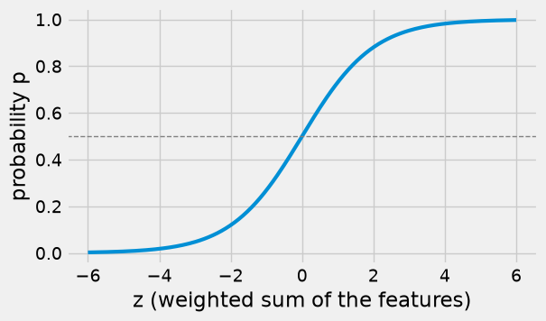
Linear regression predicts a number by adding up the features, each multiplied by a slope: \(z = b_0 + b_1 x_1 + b_2 x_2 + \cdots\). That number can be anything, such as \(-3\) or \(250\), but a probability must lie between 0 and 1. Logistic regression fixes this by passing \(z\) through the logistic function, also called the sigmoid:
The logistic function turns any number into a value between 0 and 1. When \(z = 0\), \(p = 0.5\); large positive \(z\) gives \(p\) close to 1, and large negative \(z\) gives \(p\) close to 0.
def logistic(z):
    return 1 / (1 + np.exp(-z))

z = np.linspace(-6, 6, 200)

fig, ax = plt.subplots(figsize=(6, 3.5))
ax.plot(z, logistic(z), lw=3)
ax.axhline(0.5, color='gray', lw=1, ls='--')
ax.set_xlabel('z (weighted sum of the features)')
ax.set_ylabel('probability p')
plt.show()
Here is the curve in action with a single feature. Fit logistic regression to predict a purchase from the exit rate alone. Then group the training sessions by exit rate and compare the model’s predicted probability at each group’s average exit rate with the actual purchase rate in the group.
exit_model = LogisticRegression()
exit_model.fit(X_train[['exit_rate']], y_train)

bands = pd.cut(X_train['exit_rate'], [-0.001, 0.005, 0.01, 0.02, 0.03, 0.05, 0.1, 0.15, 0.3])
summary = pd.DataFrame({'exit_rate': X_train['exit_rate'], 'purchase': y_train}).groupby(bands, observed=True).agg(
    sessions=('purchase', 'size'),
    average_exit_rate=('exit_rate', 'mean'),
    actual_purchase_rate=('purchase', 'mean'))

by_band = summary.reset_index(drop=True)
by_band['predicted probability'] = exit_model.predict_proba(
    by_band[['average_exit_rate']].rename(columns={'average_exit_rate': 'exit_rate'}))[:, 1]
by_band.round(3)
| sessions | average_exit_rate | actual_purchase_rate | predicted probability | |
|---|---|---|---|---|
| 0 | 497 | 0.003 | 0.296 | 0.211 |
| 1 | 853 | 0.008 | 0.260 | 0.202 |
| 2 | 2041 | 0.015 | 0.230 | 0.188 |
| 3 | 1535 | 0.025 | 0.180 | 0.172 |
| 4 | 1696 | 0.040 | 0.096 | 0.149 |
| 5 | 1225 | 0.074 | 0.043 | 0.105 |
| 6 | 222 | 0.128 | 0.009 | 0.059 |
| 7 | 562 | 0.197 | 0.005 | 0.027 |
grid = pd.DataFrame({'exit_rate': np.linspace(0, 0.2, 100)})

fig, ax = plt.subplots(figsize=(6, 3.5))
ax.plot(grid['exit_rate'], exit_model.predict_proba(grid)[:, 1], lw=3, label='logistic regression')
ax.scatter(by_band['average_exit_rate'], by_band['actual_purchase_rate'], s=60, color='darkorange',
           zorder=5, label='actual purchase rate')
ax.set_xlabel('exit rate')
ax.set_ylabel('probability of a purchase')
ax.legend(loc='upper right')
plt.show()
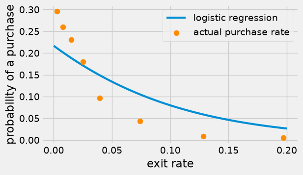
The predicted probability falls along an S-shaped curve as the exit rate rises, from about 0.21 at an exit rate near 0 to about 0.03 at 0.2. (Over this narrow range, only the right-hand part of the S shows.) The actual purchase rates fall in the same direction, but faster than the curve: the curve is too low for sessions with very low exit rates (0.21 predicted against 0.30 actual) and too high for sessions with high exit rates (0.03 predicted against 0.005). One feature alone gives a rough fit; the next subsection uses all three.
### Exercise: The Logistic Function
#   1. Write ex_logistic(z) = 1 / (1 + e^(-z)) using np.exp.
#   2. Apply it to the array ex_z and print the results rounded to 3 decimals.
# Print exactly:
# [0.018 0.269 0.5   0.731 0.982]
ex_z = np.array([-4, -1, 0, 1, 4])
### Your code starts here.


### Your code ends here.
[0.018 0.269 0.5 0.731 0.982]
15.3.2. Fitting LogisticRegression#
Fitting logistic regression with all three features follows the same fit pattern as every other scikit-learn model. Behind the scenes, fit searches for the intercept and coefficients that make the observed purchase outcomes in the training set as likely as possible.
logit = LogisticRegression()
logit.fit(X_train, y_train)

coefficients = pd.DataFrame({'coefficient': logit.coef_[0].round(3)}, index=features)
print('Intercept:', logit.intercept_.round(3))
coefficients
Intercept: [-2.441]
| coefficient | |
|---|---|
| page_value | 0.088 |
| exit_rate | -5.737 |
| product_pages | 0.006 |
Reading the coefficients. Each coefficient multiplies its feature inside \(z\), so its sign tells the direction of the effect, holding the other features fixed:
A positive coefficient means that larger values of the feature raise \(z\) and therefore raise the predicted probability of a purchase.
A negative coefficient means that larger values lower the probability.
Here page value and the number of product pages have positive coefficients (sessions that see valuable pages and view more products are more likely to end in a purchase), while the exit rate has a negative one (sessions on pages that visitors often leave are less likely to). These directions match the group averages in Section Nearest Neighbors with scikit-learn.
The size of a coefficient is harder to read than in linear regression, because the logistic curve is not a straight line: the same change in \(z\) moves the probability a lot near 50% and only a little near 0% or 100%. (Statisticians translate coefficients into changes in the odds of a purchase; that is beyond this introduction.) The coefficients also depend on each feature’s units, so do not compare their sizes across features unless the features have been scaled. The exit rate’s coefficient, \(-5.737\), looks huge next to \(0.006\) for product pages, but the exit rate only ranges from 0 to 0.2 while the page count runs to 705; each extra 0.1 of exit rate lowers \(z\) by about 0.57, and each extra 100 product pages raises it by about 0.6.
The clearest way to see what the model says is to compare predicted probabilities for sessions that differ in one feature. Here are five sessions with an exit rate of 0.02 and 30 product pages, whose pages have page values from $0 to $40.
what_if = pd.DataFrame({'page_value': [0.0, 10.0, 20.0, 30.0, 40.0],
                        'exit_rate': [0.02] * 5,
                        'product_pages': [30] * 5})
what_if['probability of purchase'] = logit.predict_proba(what_if[features])[:, 1].round(3)
what_if
| page_value | exit_rate | product_pages | probability of purchase | |
|---|---|---|---|---|
| 0 | 0.0 | 0.02 | 30 | 0.086 |
| 1 | 10.0 | 0.02 | 30 | 0.184 |
| 2 | 20.0 | 0.02 | 30 | 0.352 |
| 3 | 30.0 | 0.02 | 30 | 0.566 |
| 4 | 40.0 | 0.02 | 30 | 0.758 |
A session whose pages have a page value of $0 has a predicted probability of purchase of only 9%, and $40 raises it to 76%. The steps are uneven: going from $0 to $10 raises the probability by 10 points, from $20 to $30 by 21 points, and from $30 to $40 by 19 points. How much a feature changes the probability depends on where the session sits on the curve.
### Exercise: A Two-Feature Model
#   1. Fit a LogisticRegression on X_train[['page_value', 'exit_rate']] and y_train.
#   2. Print the two coefficients rounded to 3 decimals.
#   3. Print whether each one raises or lowers the probability of a purchase.
# Print exactly:
# page_value: 0.087 (raises purchase probability)
# exit_rate: -6.902 (lowers purchase probability)
### Your code starts here.


### Your code ends here.
page_value: 0.087 (raises purchase probability)
exit_rate: -6.902 (lowers purchase probability)
15.3.3. Predicted Probabilities#
For each session, the fitted model’s predict_proba method returns one column per class: the probability of class 0 (no purchase) and of class 1 (purchase). Each row adds up to 1. You usually keep the second column, the probability of the positive class.
proba = logit.predict_proba(X_test)
print(proba[:5].round(3))

p_buy = proba[:, 1]
[[0.921 0.079]
 [0.973 0.027]
 [0.878 0.122]
 [0.134 0.866]
 [0.964 0.036]]
test_view = X_test.copy()
test_view['p_buy'] = p_buy.round(3)
test_view['predicted'] = logit.predict(X_test)
test_view['actual'] = y_test
test_view.head(8)
| page_value | exit_rate | product_pages | p_buy | predicted | actual | |
|---|---|---|---|---|---|---|
| 5218 | 0.000000 | 0.016667 | 12 | 0.079 | 0 | 0 |
| 421 | 0.000000 | 0.200000 | 1 | 0.027 | 0 | 0 |
| 5110 | 5.694121 | 0.042323 | 34 | 0.122 | 0 | 0 |
| 6614 | 45.711463 | 0.009091 | 55 | 0.866 | 1 | 1 |
| 1817 | 0.000000 | 0.150000 | 4 | 0.036 | 0 | 0 |
| 5654 | 0.000000 | 0.111111 | 9 | 0.046 | 0 | 0 |
| 4549 | 0.000000 | 0.026500 | 34 | 0.085 | 0 | 0 |
| 12122 | 0.000000 | 0.021839 | 231 | 0.245 | 0 | 0 |
The predict method turns each probability into a label using a cutoff of 0.5: “purchase” when the probability is above 0.5, otherwise “no purchase” (a probability of exactly 0.5 almost never occurs). You can check that this is exactly what it does.
print('predict matches p_buy > 0.5:', np.array_equal(logit.predict(X_test), (p_buy > 0.5).astype(int)))
print('Test accuracy:', round(logit.score(X_test, y_test), 3))
predict matches p_buy > 0.5: True
Test accuracy: 0.885
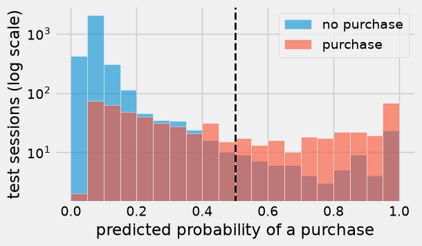
A histogram of the predicted probabilities, split by what actually happened, shows how well the model separates the two groups. The vertical axis is on a log scale so that the small bars can be seen. Sessions without a purchase mostly get low probabilities, below 0.2. Buyers are split: some get probabilities near 1, but many get low ones, and only 222 of the 572 buyers (39%) are above the 0.5 line.
fig, ax = plt.subplots(figsize=(6, 3.5))
bins = np.arange(0, 1.05, 0.05)
ax.hist(p_buy[y_test == 0], bins=bins, alpha=0.6, label='no purchase', ec='white')
ax.hist(p_buy[y_test == 1], bins=bins, alpha=0.6, label='purchase', ec='white')
ax.axvline(0.5, color='k', lw=2, ls='--')
ax.set_xlabel('predicted probability of a purchase')
ax.set_ylabel('test sessions (log scale)')
ax.set_yscale('log')
ax.legend()
plt.show()
### Exercise: Likely Buyers
#   1. Using p_buy (the test-set purchase probabilities), count the test sessions
#      whose predicted probability of a purchase is above 0.7.
#   2. Among those sessions, compute the share that actually ended in a purchase
#      (use y_test), rounded to 3 decimals.
# Print exactly:
# Likely buyers: 214
# Share who bought: 0.776
### Your code starts here.


### Your code ends here.
Likely buyers: 214
Share who bought: 0.776
15.3.4. Changing the Decision Threshold#
The cutoff of 0.5 is called the decision threshold. Nothing forces you to use 0.5. Lowering the threshold flags more sessions: recall goes up (more buyers are caught) and precision usually goes down (more false alarms). Raising it does the opposite. Which threshold is best depends on the costs from Section Evaluating Classifiers: a missed buyer costs $30 and a false alarm $3, both assumptions made for that example.
rows = []
for threshold in [0.05, 0.1, 0.15, 0.2, 0.3, 0.4, 0.5]:
    flagged = (p_buy >= threshold).astype(int)
    tn, fp, fn, tp = confusion_matrix(y_test, flagged).ravel()
    rows.append({'threshold': threshold,
                 'flagged': tp + fp,
                 'FP': fp, 'FN': fn,
                 'accuracy': round(accuracy_score(y_test, flagged), 3),
                 'precision': round(precision_score(y_test, flagged), 3),
                 'recall': round(recall_score(y_test, flagged), 3),
                 'error cost ($)': error_cost(y_test, flagged)})

thresholds = pd.DataFrame(rows)
thresholds
| threshold | flagged | FP | FN | accuracy | precision | recall | error cost ($) | |
|---|---|---|---|---|---|---|---|---|
| 0 | 0.05 | 3279 | 2709 | 2 | 0.267 | 0.174 | 0.997 | 8187 |
| 1 | 0.10 | 1154 | 657 | 75 | 0.802 | 0.431 | 0.869 | 4221 |
| 2 | 0.15 | 789 | 354 | 137 | 0.867 | 0.551 | 0.760 | 5172 |
| 3 | 0.20 | 627 | 240 | 185 | 0.885 | 0.617 | 0.677 | 6270 |
| 4 | 0.30 | 476 | 160 | 256 | 0.888 | 0.664 | 0.552 | 8160 |
| 5 | 0.40 | 370 | 102 | 304 | 0.890 | 0.724 | 0.469 | 9426 |
| 6 | 0.50 | 298 | 76 | 350 | 0.885 | 0.745 | 0.388 | 10728 |
fig, ax = plt.subplots(figsize=(6, 3.5))
ax.plot(thresholds['threshold'], thresholds['error cost ($)'], marker='o', lw=2)
ax.set_xlabel('decision threshold')
ax.set_ylabel('total error cost ($)')
plt.show()
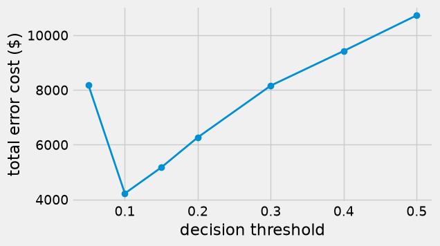
At the default threshold of 0.5, the errors cost $10,728, more than the $9,381 of flagging every session (Section Evaluating Classifiers), because only 39% of the buyers are caught. Lowering the threshold to 0.1 flags 1,154 sessions instead of 298, raises recall from 0.39 to 0.87, and cuts the error cost to $4,221, a saving of more than $6,500 on 3,699 sessions, even though accuracy falls from 0.885 to 0.802. The retailer sends more nudges that turn out to be unnecessary, but each one is cheap compared with a lost sale. Going too far does not help: at 0.05 almost every session is flagged (3,279 of 3,699) and the cost rises again to $8,187. Notice also that the most accurate threshold (0.4, with accuracy 0.890) costs $9,426, more than twice the cost at 0.1.
There is a simple rule of thumb behind this. Flag a session when the expected cost of not flagging is larger than the cost of flagging:
If the probabilities are accurate, the cost-minimizing threshold is the false-alarm cost divided by the sum of the two costs, about 0.09 here, which is close to the 0.1 that the table shows to be cheapest. As with \(k\) in Section Nearest Neighbors with scikit-learn, a careful analysis would choose the threshold on a validation set and confirm it on the test set.
### Exercise: A Threshold of 0.25
#   1. Flag the test sessions whose p_buy is at least 0.25.
#   2. Print the number flagged, the recall rounded to 3 decimals, and the
#      total error cost with error_cost(y_test, ex_flagged).
# Print exactly:
# Flagged: 542
# Recall: 0.607
# Error cost: 7335
### Your code starts here.


### Your code ends here.
Flagged: 542
Recall: 0.607
Error cost: 7335
15.3.5. Comparing with Nearest Neighbors#
A nearest neighbor classifier (kNN, short for \(k\)-nearest neighbors) can also report a probability: predict_proba gives the share of the \(k\) neighbors in each class. With \(k = 11\), the possible probabilities are \(0/11, 1/11, \ldots, 11/11\). So you can compare the two classifiers on the same test set, both at the usual threshold of 0.5 and at a lower threshold suited to the costs.
knn = make_pipeline(StandardScaler(), KNeighborsClassifier(n_neighbors=11))
knn.fit(X_train, y_train)
p_buy_knn = knn.predict_proba(X_test)[:, 1]

def summarize(name, probabilities, threshold):
    flagged = (probabilities >= threshold).astype(int)
    return {'classifier': name, 'threshold': threshold,
            'accuracy': round(accuracy_score(y_test, flagged), 3),
            'precision': round(precision_score(y_test, flagged), 3),
            'recall': round(recall_score(y_test, flagged), 3),
            'error cost ($)': error_cost(y_test, flagged)}

pd.DataFrame([summarize('kNN (k = 11)', p_buy_knn, 0.5),
              summarize('logistic regression', p_buy, 0.5),
              summarize('kNN (k = 11)', p_buy_knn, 0.1),
              summarize('logistic regression', p_buy, 0.1)])
| classifier | threshold | accuracy | precision | recall | error cost ($) | |
|---|---|---|---|---|---|---|
| 0 | kNN (k = 11) | 0.5 | 0.888 | 0.667 | 0.554 | 8124 |
| 1 | logistic regression | 0.5 | 0.885 | 0.745 | 0.388 | 10728 |
| 2 | kNN (k = 11) | 0.1 | 0.811 | 0.441 | 0.830 | 4713 |
| 3 | logistic regression | 0.1 | 0.802 | 0.431 | 0.869 | 4221 |
At the usual threshold of 0.5 the two classifiers are close in accuracy (0.888 for nearest neighbors against 0.885), but nearest neighbors catches many more buyers (recall 0.554 against 0.388) and so has the lower error cost ($8,124 against $10,728). At a threshold of 0.1, which the cost rule suggests, both become much cheaper, and logistic regression is the cheaper of the two ($4,221 against $4,728). Both then beat the $9,381 of flagging every session. So neither method wins everywhere: the exercise below shows nearest neighbors ahead at a threshold of 0.2. On this real data set the two methods are close, and the choice of threshold matters more than the choice of method. Logistic regression draws one smooth curve in each feature, which may not suit a feature such as page value, where most sessions sit at exactly 0 (Section Classification).
Beyond the numbers, the two methods have different strengths:
Logistic regression gives smooth probabilities, coefficients whose signs explain the direction of each feature’s effect, and fast predictions. It assumes that the probability changes smoothly and in one direction as each feature grows.
Nearest neighbors makes no such assumption and can follow irregular patterns, but it offers no coefficients to explain its predictions, needs scaled features, and must search the whole training set for every prediction.
In practice, analysts often try both, compare them on validation data with the measure that matters to the business, and choose a threshold to match the costs.
### Exercise: Compare at a Threshold of 0.2
#   1. Flag test sessions at a threshold of 0.2, once with p_buy (logistic regression)
#      and once with p_buy_knn (11-nearest neighbors).
#   2. Print the error cost of each with error_cost(y_test, ex_flagged), and the name
#      of the cheaper classifier.
# Print exactly:
# logistic regression cost: 6270
# kNN cost: 5079
# Cheaper: kNN
### Your code starts here.


### Your code ends here.
logistic regression cost: 6270
kNN cost: 5076
Cheaper: kNN