

16.2. K-Means Workflow#
Clustering Concepts described clustering as a way to find groups when no labels exist. This section shows how the most common method, k-means, finds those groups. It first works through the method in words, then runs it by hand with NumPy on real customer data, and finally lets scikit-learn do the same work in one call.
16.2.1. How K-Means Works#
K-means needs one decision from you before it starts: the number of clusters, called k. Each cluster is summarized by a centroid, a point whose coordinates are the average of the cluster’s members on every feature. You can think of the centroid as the cluster’s center of gravity.
The method alternates between two simple moves.
Choose k starting centroids.
Assignment step: give every observation to the cluster whose centroid is closest, using straight-line (Euclidean) distance.
Update step: move each centroid to the average position of the observations now assigned to it.
Repeat steps 2 and 3 until the assignments stop changing.
When a full round changes no assignment, the algorithm has reached convergence. The centroids can no longer move, so more rounds would only repeat the same result.
What does k-means try to achieve? Each observation lies some distance from its own centroid, and how spread out the points are around their centroids is the within-cluster variation. The within-cluster sum of squares measures it by adding up the squared distances from every observation to its centroid. A small value means the clusters are compact. Both steps can only lower this total or leave it unchanged, which is why the process always settles. It may settle on a good arrangement that is not the best possible one, a point covered again under initialization.
16.2.2. A Wholesale Customer Example#
A wholesale distributor in Portugal sells to hotels, restaurants, and cafes, and also to retail stores. The wholesale_customers.csv file describes 440 of its clients. For each client it records the annual spending, in monetary units, on six product groups (the source does not name the currency), along with the client’s sales channel and region. The data are real: they come from the UCI Machine Learning Repository (dataset 292, donated by Margarida Cardoso in 2014, from a study by Nuno Abreu in 2011) and are shared under a CC BY 4.0 license. This book’s version adds a client ID and replaces the numeric channel and region codes with names; the spending values are unchanged.
clients = pd.read_csv(path_data + 'wholesale_customers.csv')
clients.head()
| client_id | channel | region | fresh | milk | grocery | frozen | detergents_paper | delicatessen | |
|---|---|---|---|---|---|---|---|---|---|
| 0 | W001 | Retail | Other | 12669 | 9656 | 7561 | 214 | 2674 | 1338 |
| 1 | W002 | Retail | Other | 7057 | 9810 | 9568 | 1762 | 3293 | 1776 |
| 2 | W003 | Retail | Other | 6353 | 8808 | 7684 | 2405 | 3516 | 7844 |
| 3 | W004 | HoReCa | Other | 13265 | 1196 | 4221 | 6404 | 507 | 1788 |
| 4 | W005 | Retail | Other | 22615 | 5410 | 7198 | 3915 | 1777 | 5185 |
clients['channel'].value_counts()
channel
HoReCa    298
Retail    142
Name: count, dtype: int64
The channel column says whether a client is a hotel, restaurant, or cafe (HoReCa) or a retailer. K-means will not see this column. Use it only afterward, as a check.
To keep the picture simple, cluster on two product groups: grocery and detergents_paper (cleaning and paper goods). Spending on each runs from a few monetary units to tens of thousands, so most clients would be squeezed into one corner of an ordinary plot. Use a log scale instead. A base-10 logarithm turns each tenfold increase into one step: 100 becomes 2, 1,000 becomes 3, and 10,000 becomes 4. Equal distances on the plot then mean equal percentage differences in spending, which is how a manager would compare a small account with a large one. Both columns are in the same units, so neither one dominates the distance calculation. (Section Interpreting Clusters shows what to do when features are measured in different units.)
clients['log_grocery'] = np.log10(clients['grocery'])
clients['log_detergents_paper'] = np.log10(clients['detergents_paper'])
clients[['grocery', 'log_grocery', 'detergents_paper', 'log_detergents_paper']].head()
| grocery | log_grocery | detergents_paper | log_detergents_paper | |
|---|---|---|---|---|
| 0 | 7561 | 3.878579 | 2674 | 3.427161 |
| 1 | 9568 | 3.980821 | 3293 | 3.517592 |
| 2 | 7684 | 3.885587 | 3516 | 3.546049 |
| 3 | 4221 | 3.625415 | 507 | 2.705008 |
| 4 | 7198 | 3.857212 | 1777 | 3.249687 |
plt.figure(figsize=(6, 5))
plt.scatter(clients['log_grocery'], clients['log_detergents_paper'], s=18, color='gray', alpha=0.7)
plt.title('Wholesale clients: annual spending (log10 scale)')
plt.xlabel('Grocery spending (log10 of monetary units)')
plt.ylabel('Detergents and paper spending (log10 of monetary units)')
plt.show()
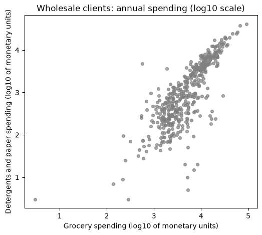
The clients form one broad cloud, with more spending on cleaning and paper goods going along with more spending on groceries. A denser band runs along the upper right, but no clear gap separates the clients into groups, so the picture alone does not settle the question a manager would ask: are there groups of clients the distributor could serve differently, for example with different delivery schedules or promotions?
### Exercise: Log Scale
# Annual spending by four clients differs by factors of 10.
#   1. Take the base-10 logarithm of each value with np.log10.
#   2. Compare the largest-to-smallest ratio before and after the logarithm.
# Print exactly:
# Logged: [2.0, 3.0, 4.0, 5.0]
# Ratio, raw: 1000.0
# Ratio, logged: 2.5
import numpy as np

ex_spend = np.array([100, 1000, 10000, 100000])
### Your code starts here.


### Your code ends here.
Logged: [2.0, 3.0, 4.0, 5.0]
Ratio, raw: 1000.0
Ratio, logged: 2.5
16.2.3. Running K-Means Step by Step#
Before using a library, run the algorithm yourself. First put the two log features into a NumPy array, one row per client.
X = clients[['log_grocery', 'log_detergents_paper']].to_numpy()
print('Shape of X:', X.shape)
Shape of X: (440, 2)
Initialization means choosing the starting centroids. A common choice is to use two actual clients. Pick two whose spending differs clearly, W145 (a smaller account) and W326 (a larger one).
start_ids = ['W145', 'W326']
start_rows = [clients.index[clients['client_id'] == cid][0] for cid in start_ids]
centers = X[start_rows].copy()
print(pd.DataFrame(centers, index=start_ids, columns=['log_grocery', 'log_detergents_paper']).round(2))
      log_grocery  log_detergents_paper
W145         3.30                  2.71
W326         4.13                  3.10
Now one round has two parts. The assignment step measures the distance from every client to each centroid and keeps the nearer one. The update step replaces each centroid with the mean of its clients. After each update the code also prints the within-cluster sum of squares and how many assignments changed. The loop stops as soon as a round changes nothing.
def assign(X, centers):
    # distance from every client (rows) to every center (columns)
    gaps = X[:, None, :] - centers[None, :, :]
    distances = np.sqrt((gaps ** 2).sum(axis=2))
    return distances.argmin(axis=1)

def update(X, labels, k):
    return np.array([X[labels == j].mean(axis=0) for j in range(k)])

def wcss(X, labels, centers):
    return ((X - centers[labels]) ** 2).sum()

start_centers = centers.copy()
history = []          # (round number, labels, centers) after each round
labels = None
for round_number in range(1, 21):
    new_labels = assign(X, centers)
    if labels is not None and (new_labels == labels).all():
        print(f'Round {round_number}: no assignment changed, so k-means has converged.')
        break
    changed = len(X) if labels is None else int((new_labels != labels).sum())
    labels = new_labels
    centers = update(X, labels, 2)
    history.append((round_number, labels, centers))
    print(f'Round {round_number}: {changed:3d} clients (re)assigned, '
          f'within-cluster sum of squares = {wcss(X, labels, centers):.3f}')
Round 1: 440 clients (re)assigned, within-cluster sum of squares = 137.641
Round 2:  19 clients (re)assigned, within-cluster sum of squares = 129.816
Round 3:   4 clients (re)assigned, within-cluster sum of squares = 129.537
Round 4:   1 clients (re)assigned, within-cluster sum of squares = 129.510
Round 5:   1 clients (re)assigned, within-cluster sum of squares = 129.497
Round 6: no assignment changed, so k-means has converged.
In round 1 every client is assigned for the first time. The total falls from 137.641 to 129.816 in round 2, when 19 clients switch sides, and then by smaller amounts (0.279, 0.027, and 0.013) as four, one, and one clients move. In round 6 no assignment changes, so the process stops. The plots below show the clients colored by their group after four of the rounds, with the updated centroids marked by black X symbols. In the first panel, white diamonds mark the two starting centroids.
colors = ['tab:green', 'tab:purple']
shown = [history[0], history[1], history[2], history[-1]]

fig, axes = plt.subplots(2, 2, figsize=(10, 9), sharex=True, sharey=True)
for ax, (round_number, lab, cen) in zip(axes.ravel(), shown):
    for j in range(2):
        ax.scatter(X[lab == j, 0], X[lab == j, 1], s=14, color=colors[j], alpha=0.7)
    ax.scatter(cen[:, 0], cen[:, 1], marker='X', s=200, color='black', edgecolor='white')
    if round_number == 1:
        ax.scatter(start_centers[:, 0], start_centers[:, 1], marker='D', s=90, color='white', edgecolor='black')
    ax.set_title(f'After round {round_number}')
for ax in axes[1]:
    ax.set_xlabel('Grocery (log10)')
for ax in axes[:, 0]:
    ax.set_ylabel('Detergents and paper (log10)')
plt.tight_layout()
plt.show()
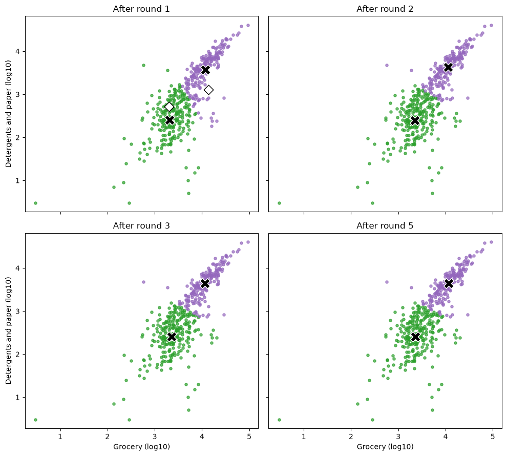
The cloud has a dense band of high-spending clients along the upper right and a looser, lower-spending mass below and to the left. After round 1, the upper centroid already sits in the band and the lower one in the looser mass. The later rounds move the centroids only slightly and shift a few clients near the dividing line between the groups, so the first and last panels look alike. Colors are only labels: the green group could just as well have been purple.
final_centers = history[-1][2]
final_labels = history[-1][1]
print('Final centers in log units:')
print(pd.DataFrame(final_centers, columns=['log_grocery', 'log_detergents_paper'], index=['group 0', 'group 1']).round(3))
print('Clients per group:', np.bincount(final_labels))
Final centers in log units:
         log_grocery  log_detergents_paper
group 0        3.363                 2.409
group 1        4.061                 3.649
Clients per group: [249 191]
The hand-run result is two groups, a larger lower-spending group and a smaller higher-spending group. The same result takes a few lines of library code, shown next.
### Exercise: Within-Cluster Sum of Squares
# K-means has put six orders (sizes in dollars) into two clusters with these centers.
#   1. Compute each order's squared distance to the center of its own cluster.
#   2. Add the squared distances to get the within-cluster sum of squares.
# Print exactly:
# Within-cluster sum of squares: 40
ex_sizes = [5, 7, 9, 21, 25, 29]
ex_labels = [0, 0, 0, 1, 1, 1]
ex_centers = [7, 25]
### Your code starts here.


### Your code ends here.
Within-cluster sum of squares: 40
16.2.4. K-Means with scikit-learn#
scikit-learn’s KMeans follows the same fit pattern used for regression and classification: create the model, call .fit on the features, and then read the results. Two settings control the starting centroids. By default, KMeans picks starting points at random (with a rule that tends to spread them apart), so two runs can begin in different places and, now and then, end in different clusters. The setting n_init tells it how many different starts to try; it keeps the run with the smallest within-cluster sum of squares. The setting random_state fixes the random number generator, so that everyone who runs the code gets the same answer.
model = KMeans(n_clusters=2, n_init=10, random_state=12)
model.fit(X)

print('Centers in log units:')
print(model.cluster_centers_.round(3))
print('First 10 labels:', model.labels_[:10])
print('Clients per cluster:', np.bincount(model.labels_))
print('Within-cluster sum of squares:', round(model.inertia_, 3))
Centers in log units:
[[3.367 2.416]
 [4.066 3.659]]
First 10 labels: [1 1 1 0 1 1 1 1 1 1]
Clients per cluster: [252 188]
Within-cluster sum of squares: 129.491
cluster_centers_ holds one row per cluster, in the same log units as the features, and labels_ gives each client’s cluster number. scikit-learn calls the within-cluster sum of squares inertia_. Log units are hard to read, so convert the centers back to monetary units with 10 ** center.
centers_money = pd.DataFrame(10 ** model.cluster_centers_,
                             columns=['grocery', 'detergents_paper'])
centers_money.round(0)
| grocery | detergents_paper | |
|---|---|---|
| 0 | 2330.0 | 261.0 |
| 1 | 11647.0 | 4560.0 |
Each center is an average of logarithms, so converting it back gives a cluster’s typical (geometric mean) spending, not the arithmetic average of the monetary amounts. One cluster typically spends far more on both product groups than the other.
Finally, compare with the hand-run result. Cluster numbers may be swapped, so line up each scikit-learn center with the nearest center from the hand-run loop.
compare = pd.DataFrame({
    'by hand (grocery)': 10 ** final_centers[:, 0],
    'by hand (detergents_paper)': 10 ** final_centers[:, 1],
})
order = [np.argmin(((model.cluster_centers_ - c) ** 2).sum(axis=1)) for c in final_centers]
compare['sklearn (grocery)'] = 10 ** model.cluster_centers_[order, 0]
compare['sklearn (detergents_paper)'] = 10 ** model.cluster_centers_[order, 1]
print(compare.round(0))
print('Largest difference in log units:', np.abs(final_centers - model.cluster_centers_[order]).max().round(6))
print('Clients grouped differently:', int((final_labels != np.array(order)[model.labels_]).sum()))
   by hand (grocery)  by hand (detergents_paper)  sklearn (grocery)  \
0             2305.0                       256.0             2330.0
1            11516.0                      4454.0            11647.0

   sklearn (detergents_paper)
0                       261.0
1                      4560.0
Largest difference in log units: 0.010193
Clients grouped differently: 3
The two sets of centers are very close, within about 0.01 in log units, and the within-cluster sum of squares differs only in the third decimal place (129.497 by hand, 129.491 from scikit-learn). They are not identical: 3 clients near the boundary are grouped differently, because the two runs stopped at slightly different arrangements. The step-by-step version started from two particular clients. KMeans tried ten starts and kept the one with the smallest sum. Here the two approaches end in nearly the same place, which suggests that the grouping is stable for these data. With harder data the starts can disagree by more, which is why n_init matters.
### Exercise: Fit K-Means with scikit-learn
# Six stores are described by two features: weekly foot traffic (hundreds) and average basket (dollars, tens).
#   1. Fit KMeans with 2 clusters, n_init=10, and random_state=0.
#   2. Count the stores in each cluster, sorted from smallest to largest.
#   3. Round the cluster centers to 2 decimals and sort them.
# Print exactly:
# Cluster sizes: [3, 3]
# Centers: [[1.33, 3.0], [9.0, 9.0]]
import numpy as np
from sklearn.cluster import KMeans

ex_X = np.array([[1, 2], [1, 4], [2, 3], [8, 8], [9, 10], [10, 9]])
### Your code starts here.


### Your code ends here.
Cluster sizes: [3, 3]
Centers: [[1.33, 3.0], [9.0, 9.0]]
16.2.5. Checking Against the Known Channel#
K-means never saw the channel column, so the channel gives an independent check. If the clusters are meaningful, they should line up with the channel to a good degree. A cross-tabulation counts how many clients fall in each pair of cluster and channel.
clients['cluster'] = model.labels_
pd.crosstab(clients['cluster'], clients['channel'])
| channel | HoReCa | Retail |
|---|---|---|
| cluster | ||
| 0 | 246 | 6 |
| 1 | 52 | 136 |
table = pd.crosstab(clients['cluster'], clients['channel'])
majority = table.idxmax(axis=0)       # for each channel, its most common cluster
print('Majority cluster for each channel:')
print(majority)

matches = clients['cluster'] == clients['channel'].map(majority)
print('Clients whose cluster matches their channel:', matches.sum(), 'of', len(clients))
print('Share:', round(matches.mean(), 3))
print()
print('Share of each channel found in its majority cluster:')
print((table.max(axis=0) / table.sum(axis=0)).round(3))
Majority cluster for each channel:
channel
HoReCa    0
Retail    1
dtype: int32
Clients whose cluster matches their channel: 382 of 440
Share: 0.868

Share of each channel found in its majority cluster:
channel
HoReCa    0.826
Retail    0.958
dtype: float64
The table shows that most Retail clients fall in one cluster and most HoReCa clients in the other. Counting the clients whose cluster matches the majority cluster of their channel, 382 of 440 clients (86.8%) agree: 82.6% of HoReCa clients and 95.8% of Retail clients.
The cluster numbers are arbitrary names. Which group gets 0 and which gets 1 depends on the starting centroids, so cluster 1 is not “better” or “bigger” than cluster 0. Rerunning with another seed may swap the numbers and leave the groups unchanged. That is why each channel is matched to its most common cluster instead of assuming that cluster 0 means HoReCa. To see this, rerun with a different seed.
other = KMeans(n_clusters=2, n_init=10, random_state=99).fit(X)
agree = int((other.labels_ == model.labels_).sum())
print('Clients with the same cluster number under seed 99 and seed 12:', agree)
print('Clients grouped the same way, ignoring the names:', max(agree, len(X) - agree))
Clients with the same cluster number under seed 99 and seed 12: 0
Clients grouped the same way, ignoring the names: 440
fig, axes = plt.subplots(1, 2, figsize=(11, 5), sharex=True, sharey=True)

channel_colors = {'HoReCa': 'tab:blue', 'Retail': 'tab:orange'}
for name, color in channel_colors.items():
    part = clients[clients['channel'] == name]
    axes[0].scatter(part['log_grocery'], part['log_detergents_paper'], s=16, color=color, alpha=0.7, label=name)
axes[0].set_title('Colored by known channel')
axes[0].legend()

cluster_colors = ['tab:green', 'tab:purple']
for j in range(2):
    part = clients[clients['cluster'] == j]
    axes[1].scatter(part['log_grocery'], part['log_detergents_paper'], s=16, color=cluster_colors[j], alpha=0.7, label=f'Cluster {j}')
axes[1].scatter(model.cluster_centers_[:, 0], model.cluster_centers_[:, 1], marker='X', s=200, color='black', edgecolor='white')
axes[1].set_title('Colored by k-means cluster')
axes[1].legend()

for ax in axes:
    ax.set_xlabel('Grocery (log10)')
axes[0].set_ylabel('Detergents and paper (log10)')
plt.tight_layout()
plt.show()
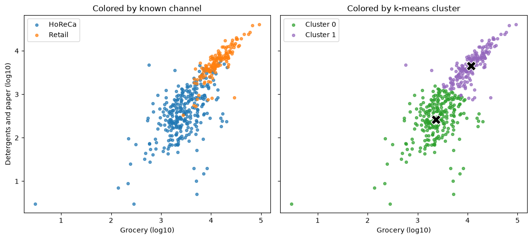
In the left panel, Retail clients (orange) fill the dense upper-right band, while HoReCa clients (blue) spread over the lower-spending mass and also reach into the band’s edge. In the right panel, k-means splits the cloud with a straight diagonal boundary. The misses are the clients on the other side of that boundary from most of their channel: 52 HoReCa clients who fall in the higher-spending cluster and 6 Retail clients who fall in the lower-spending one. The next output compares their typical spending with the clients that k-means matched correctly.
misses = clients[~matches]
print('Misses by channel:')
print(misses['channel'].value_counts())
print()
print('Median spending (monetary units):')
summary = pd.DataFrame({
    'HoReCa misses': misses[misses['channel'] == 'HoReCa'][['grocery', 'detergents_paper']].median(),
    'HoReCa matched': clients[matches & (clients['channel'] == 'HoReCa')][['grocery', 'detergents_paper']].median(),
    'Retail matched': clients[matches & (clients['channel'] == 'Retail')][['grocery', 'detergents_paper']].median(),
})
print(summary.round(0))
Misses by channel:
channel
HoReCa    52
Retail     6
Name: count, dtype: int64

Median spending (monetary units):
                  HoReCa misses  HoReCa matched  Retail matched
grocery                  7320.0          2405.0         12898.0
detergents_paper         2252.0           289.0          5967.0
The misses are mostly HoReCa clients: 52 of the 58. The median spending of those 52, 7,320 on groceries and 2,252 on detergents and paper, lies between the two matched groups. On the log scale that k-means uses, it is closer to the Retail clients’ (12,898 and 5,967) than to the matched HoReCa clients’ (2,405 and 289). In other words, they buy more like retailers. For the distributor, this is a useful finding rather than only an error. Suppose a promotion for retail-like buyers, such as a bulk discount on cleaning and paper goods, is aimed at the cluster instead of at the Retail channel. It would reach the retailers, and also the hotels, restaurants, and cafes that buy like retailers. Those clients may well respond to the offer, so the cluster may describe buying behavior better than the channel label does. On the other hand, the lower-spending cluster contains 6 Retail clients who buy lightly and would be left out. Whether that is acceptable depends on the cost of a wasted offer compared with the cost of a missed one.
Agreement with a known label is also a luxury. In most business problems no channel column exists, and the analyst must judge the groups by whether they make sense and support a decision. Two questions remain open here: whether two clusters is the right number, and what happens when features are measured in different units. Section Interpreting Clusters takes up scaling, the elbow and silhouette checks for choosing k, and how to describe each cluster in business terms.
### Exercise: Agreement with a Known Label
# K-means has put ten clients into two clusters, and their sales channel is known.
#   1. Cross-tabulate cluster against channel with pd.crosstab.
#   2. For each channel, find its most common cluster with idxmax(axis=0).
#   3. Count the clients whose cluster matches their channel's most common cluster.
# Print exactly:
# Matches: 8 of 10
# Share: 0.8
import pandas as pd

ex_clients = pd.DataFrame({
    'cluster': [1, 1, 1, 0, 1, 0, 0, 0, 0, 0],
    'channel': ['Retail', 'Retail', 'Retail', 'Retail',
                'HoReCa', 'HoReCa', 'HoReCa', 'HoReCa', 'HoReCa', 'HoReCa'],
})
### Your code starts here.


### Your code ends here.
Matches: 8 of 10
Share: 0.8
16.2.6. Section Practice#
Use this short exercise to check the main workflow from this section.
### Exercise: Practice K-Means Workflow
# Run one round of k-means by hand on six customers' monthly spend (one feature).
#   1. Assign each value to the nearer of the two centers (0 or 1).
#   2. Update each center to the mean of the values assigned to it.
# Print exactly:
# Assignments: [0, 0, 0, 1, 1, 1]
# New centers: [22.0, 71.0]
ex_spend = [12, 20, 34, 58, 70, 85]
ex_centers = [20, 60]
### Your code starts here.


### Your code ends here.
Assignments: [0, 0, 0, 1, 1, 1]
New centers: [22.0, 71.0]