

16.3. Interpreting Clusters#
This section shows how to interpret a k-means result after the model has been fit. The technical output is only the starting point. The analyst still has to choose a reasonable number of clusters, describe each cluster, and decide whether the grouping supports the business question.
This section continues with the wholesale clients from K-Means Workflow. A distributor in Portugal sells to hotels, restaurants, and cafes (HoReCa) and to retail stores. For each of 440 clients, the data record annual spending, in monetary units, on six product groups: fresh food, milk, grocery, frozen food, detergents and paper goods, and delicatessen. The data are real, from the UCI Machine Learning Repository (dataset 292, CC BY 4.0), and are described in K-Means Workflow. That section clustered on two product groups. Here you use all six, and k-means does not get the channel. Sales wants to know whether the clients fall into groups that call for different treatment, such as different delivery schedules, promotions, or account managers.
clients = pd.read_csv(path_data + 'wholesale_customers.csv')
clients.head()
| client_id | channel | region | fresh | milk | grocery | frozen | detergents_paper | delicatessen | |
|---|---|---|---|---|---|---|---|---|---|
| 0 | W001 | Retail | Other | 12669 | 9656 | 7561 | 214 | 2674 | 1338 |
| 1 | W002 | Retail | Other | 7057 | 9810 | 9568 | 1762 | 3293 | 1776 |
| 2 | W003 | Retail | Other | 6353 | 8808 | 7684 | 2405 | 3516 | 7844 |
| 3 | W004 | HoReCa | Other | 13265 | 1196 | 4221 | 6404 | 507 | 1788 |
| 4 | W005 | Retail | Other | 22615 | 5410 | 7198 | 3915 | 1777 | 5185 |
spend_cols = ['fresh', 'milk', 'grocery', 'frozen', 'detergents_paper', 'delicatessen']
clients[spend_cols].describe().round(0)
| fresh | milk | grocery | frozen | detergents_paper | delicatessen | |
|---|---|---|---|---|---|---|
| count | 440.0 | 440.0 | 440.0 | 440.0 | 440.0 | 440.0 |
| mean | 12000.0 | 5796.0 | 7951.0 | 3072.0 | 2881.0 | 1525.0 |
| std | 12647.0 | 7380.0 | 9503.0 | 4855.0 | 4768.0 | 2820.0 |
| min | 3.0 | 55.0 | 3.0 | 25.0 | 3.0 | 3.0 |
| 25% | 3128.0 | 1533.0 | 2153.0 | 742.0 | 257.0 | 408.0 |
| 50% | 8504.0 | 3627.0 | 4756.0 | 1526.0 | 816.0 | 966.0 |
| 75% | 16934.0 | 7190.0 | 10656.0 | 3554.0 | 3922.0 | 1820.0 |
| max | 112151.0 | 73498.0 | 92780.0 | 60869.0 | 40827.0 | 47943.0 |
Spending is very uneven. Median spending on fresh food is about 8,500, but the largest client spends more than 112,000. Every column has a few very large clients and many small ones, and the smallest values are only 3 monetary units, so a plot or a distance in monetary units would be dominated by the large accounts.
16.3.1. Scaling the Features#
Put the features on a comparable scale first. The six columns do not have the same spread. Fresh food has a standard deviation of about 12,600 monetary units, while delicatessen has about 2,800. K-means groups points by distance, so a column with a large spread counts for more than a column with a small one, and a few huge clients can pull on the centroids. Two steps fix this. First, take the base-10 logarithm of each column, as in K-Means Workflow, so that equal distances mean equal percentage differences. Second, standardize the logged columns with StandardScaler, which subtracts each column’s mean and divides by its standard deviation, so that every feature has mean 0 and standard deviation 1. The table compares the spread of each column before and after the logarithm.
raw = clients[spend_cols]
log_spend = np.log10(raw)

pd.DataFrame({'std, monetary units': raw.std().round(0),
              'std, log10 units': log_spend.std().round(2)})
| std, monetary units | std, log10 units | |
|---|---|---|
| fresh | 12647.0 | 0.64 |
| milk | 7380.0 | 0.47 |
| grocery | 9503.0 | 0.48 |
| frozen | 4855.0 | 0.56 |
| detergents_paper | 4768.0 | 0.75 |
| delicatessen | 2820.0 | 0.57 |
In monetary units the standard deviations range from about 2,800 to 12,600, a factor of more than four. After the logarithm they are all between 0.47 and 0.75. Standardizing then makes them exactly equal. The logarithm does most of the work here, and standardizing is a safe habit that matters more whenever columns come in different units (dollars and days, say). Here is k-means with 4 clusters on the raw features and on the standardized log features, with both results plotted in monetary units on log axes:
X_scaled = StandardScaler().fit_transform(log_spend)

raw_model = KMeans(n_clusters=4, n_init=10, random_state=101).fit(raw)
raw_labels = raw_model.labels_
scaled_labels = KMeans(n_clusters=4, n_init=10, random_state=101).fit_predict(X_scaled)

print('Clients per cluster, raw features:   ', np.bincount(raw_labels))
print('Clients per cluster, scaled features:', np.bincount(scaled_labels))
print()
print('Raw-feature cluster centers (monetary units):')
print(pd.DataFrame(raw_model.cluster_centers_, columns=spend_cols).round(0))

fig, axes = plt.subplots(1, 2, figsize=(11, 4.5), sharey=True)
sns.scatterplot(data=clients, x='grocery', y='fresh', hue=raw_labels, palette='tab10', s=25, ax=axes[0])
axes[0].set_title('Raw features')
sns.scatterplot(data=clients, x='grocery', y='fresh', hue=scaled_labels, palette='tab10', s=25, ax=axes[1])
axes[1].set_title('Logged and standardized features')
for ax in axes:
    ax.set_xscale('log')
    ax.set_yscale('log')
    ax.set_xlabel('Grocery (monetary units, log axis)')
axes[0].set_ylabel('Fresh (monetary units, log axis)')
plt.tight_layout()
plt.show()
Clients per cluster, raw features:    [287  58   7  88]
Clients per cluster, scaled features: [119 130 130  61]

Raw-feature cluster centers (monetary units):
     fresh     milk  grocery  frozen  detergents_paper  delicatessen
0   8978.0   3178.0   4014.0  2766.0            1140.0        1054.0
1  36144.0   5471.0   6129.0  6299.0            1064.0        2317.0
2  25283.0  41368.0  52461.0  7779.0           24217.0        9194.0
3   4886.0  11718.0  18452.0  1567.0            8063.0        1929.0
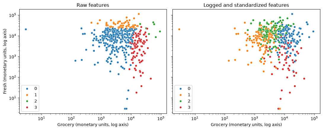
On the raw features (left), the clusters follow the largest amounts. The orange cluster holds 58 clients with very high fresh-food spending, the red cluster holds 88 clients with high grocery spending, and the green cluster holds just 7 clients, the biggest accounts of all. The remaining 287 clients (blue) form one cluster, however they spend. After the logarithm and standardizing (right), the clusters have more even sizes (61 to 130 clients), and they reflect what clients buy as well as how much. They overlap in this plot because it shows only two of the six columns that k-means used. From here on, cluster the scaled features.
### Exercise: Log and Standardize
# Annual fresh-food spending by three clients differs by factors of 10.
#   1. Take the base-10 logarithm of each value with np.log10.
#   2. Standardize the logged values: subtract their mean and divide by their
#      standard deviation (use .std(), which divides by n, as StandardScaler does).
#   3. Print both lists rounded to 2 decimals.
# Print exactly:
# Logged: [2.0, 3.0, 4.0]
# Standardized: [-1.22, 0.0, 1.22]
import numpy as np

ex_spend = np.array([100, 1000, 10000])
### Your code starts here.


### Your code ends here.
Logged: [2.0, 3.0, 4.0]
Standardized: [-1.22, 0.0, 1.22]
16.3.2. Choosing k#
K-means needs the number of clusters up front. Two common heuristics are the elbow method and the silhouette score. These tools help compare choices, but they do not remove judgment. A technically neat value of k still needs a practical interpretation.
16.3.2.1. Elbow Check#
The elbow method fits k-means for several values of k and records the model’s inertia, which is the within-cluster sum of squares. Lower inertia is better, but it always improves as k increases. The useful question is where the improvement starts to flatten.
inertias = []
k_values = range(2, 8)

for k in k_values:
    model = KMeans(n_clusters=k, n_init=10, random_state=101)
    model.fit(X_scaled)
    inertias.append(model.inertia_)

elbow_df = pd.DataFrame({"k": list(k_values), "inertia": inertias})
elbow_df
| k | inertia | |
|---|---|---|
| 0 | 2 | 1847.995021 |
| 1 | 3 | 1558.102201 |
| 2 | 4 | 1391.755317 |
| 3 | 5 | 1271.663870 |
| 4 | 6 | 1179.648219 |
| 5 | 7 | 1092.255267 |
sns.lineplot(data=elbow_df, x="k", y="inertia", marker="o")
plt.title("Elbow Check for K-Means")
plt.xlabel("Number of clusters")
plt.ylabel("Inertia");
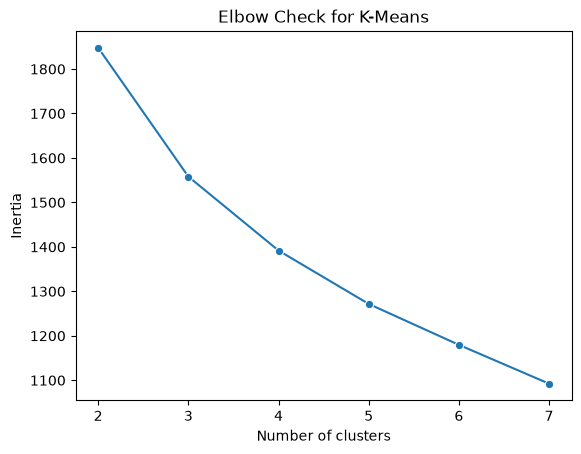
The curve falls smoothly from about 1,850 at k = 2 to about 1,090 at k = 7. Each extra cluster removes less than the one before, but there is no sharp bend where the curve suddenly flattens. The elbow does not single out a value of k.
16.3.2.2. Silhouette Check#
The silhouette score compares how close each point is to its own cluster relative to nearby clusters. Values closer to 1 suggest tighter, better-separated clusters. Values near 0 suggest overlap, and negative values suggest points may be assigned to the wrong cluster.
silhouette_scores = []

for k in k_values:
    model = KMeans(n_clusters=k, n_init=10, random_state=101)
    labels = model.fit_predict(X_scaled)
    silhouette_scores.append(silhouette_score(X_scaled, labels))

silhouette_df = pd.DataFrame({"k": list(k_values), "silhouette": silhouette_scores})
silhouette_df
| k | silhouette | |
|---|---|---|
| 0 | 2 | 0.289586 |
| 1 | 3 | 0.258485 |
| 2 | 4 | 0.187776 |
| 3 | 5 | 0.196243 |
| 4 | 6 | 0.199100 |
| 5 | 7 | 0.184499 |
sns.lineplot(data=silhouette_df, x="k", y="silhouette", marker="o")
plt.title("Silhouette Check for K-Means")
plt.xlabel("Number of clusters")
plt.ylabel("Silhouette score");
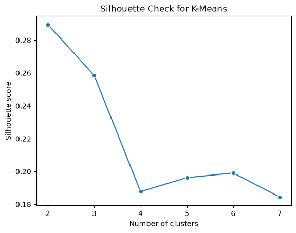
The two checks do not give a clear answer. The silhouette score is highest at k = 2 (about 0.29), next at k = 3 (about 0.26), and then falls to about 0.19 for k = 4 to 7, which are all about equally good. Every score is well below 0.5, a common rough benchmark for clearly separated clusters, which suggests that the clients form a continuous cloud rather than distinct groups, so any choice of k is a way of cutting up the cloud, not of discovering natural clusters. In real data, the two checks often disagree or show no clear winner, and the business question has to break the tie.
Here, k = 2 mostly recreates the split between hotels, restaurants, and cafes and retailers, which the distributor already has in its records. It would tell the sales team little that is new. This section chooses k = 4 because it is a number of segments a sales team can manage and because, as the next section shows, the four groups differ in what they buy in ways that call for different actions. Its silhouette score is lower than for k = 2 or 3, and about the same as for k = 5 or 6, so treat the segments as a convenient way to organize the clients and check that they are stable.
### Exercise: Compute a Silhouette Value
# One client at spending level 3 sits in a cluster with clients at 1 and 5.
# The nearest other cluster holds clients at 9, 11, and 13.
#   1. a = mean distance from the client to the other members of its own cluster.
#   2. b = mean distance from the client to the members of the other cluster.
#   3. silhouette = (b - a) / max(a, b).
# Print exactly:
# a: 2.0
# b: 8.0
# Silhouette: 0.75
x = 3
own = [1, 5]
other = [9, 11, 13]
### Your code starts here.


### Your code ends here.
a: 2.0
b: 8.0
Silhouette: 0.75
16.3.3. Describing Clusters#
After choosing k, summarize each cluster in the units that matter for the decision. The model is fit on the standardized log features, but the clusters are described in the original units, monetary units of annual spending, because those are what a manager can act on. Because a few very large clients would distort an average, use the median of each column. In a customer example, other useful summaries might be purchase frequency, tenure, or churn rate. In an operations example, they might be processing time, defect rate, and order size.
final_model = KMeans(n_clusters=4, n_init=10, random_state=101)
clients['cluster'] = final_model.fit_predict(X_scaled)

profile = clients.groupby('cluster')[spend_cols].median().round(0)
profile['clients'] = clients['cluster'].value_counts().sort_index()
profile
| fresh | milk | grocery | frozen | detergents_paper | delicatessen | clients | |
|---|---|---|---|---|---|---|---|
| cluster | |||||||
| 0 | 7842.0 | 8384.0 | 12311.0 | 1365.0 | 4621.0 | 1682.0 | 119 |
| 1 | 7814.0 | 1112.0 | 1820.0 | 1386.0 | 224.0 | 432.0 | 130 |
| 2 | 16978.0 | 3122.0 | 3430.0 | 4324.0 | 515.0 | 1374.0 | 130 |
| 3 | 1073.0 | 6964.0 | 10518.0 | 340.0 | 4508.0 | 295.0 | 61 |
The raw medians are hard to compare across columns, because a typical client spends much more on fresh food than on delicatessen. Dividing each cluster’s median by the median of all 440 clients shows which products a cluster buys more or less than the typical client. A value of 2 means twice the overall median, and 0.5 means half.
relative = (profile[spend_cols] / clients[spend_cols].median()).round(2)
relative
| fresh | milk | grocery | frozen | detergents_paper | delicatessen | |
|---|---|---|---|---|---|---|
| cluster | ||||||
| 0 | 0.92 | 2.31 | 2.59 | 0.89 | 5.66 | 1.74 |
| 1 | 0.92 | 0.31 | 0.38 | 0.91 | 0.27 | 0.45 |
| 2 | 2.00 | 0.86 | 0.72 | 2.83 | 0.63 | 1.42 |
| 3 | 0.13 | 1.92 | 2.21 | 0.22 | 5.52 | 0.31 |
16.3.4. Practical Interpretation#
Cluster labels are useful only when they support an interpretable decision. The final step is to describe the groups in business language and decide whether the segments suggest different actions.
The colors in a cluster plot are arbitrary. Cluster 0 in one model is not guaranteed to match cluster 0 in another model, even when the same data are used.
sns.scatterplot(data=clients, x='grocery', y='fresh', hue='cluster', palette='tab10', s=25)
plt.xscale('log')
plt.yscale('log')
plt.xlabel('Grocery (monetary units, log axis)')
plt.ylabel('Fresh (monetary units, log axis)')
plt.title('Wholesale Client Segments')
plt.show()
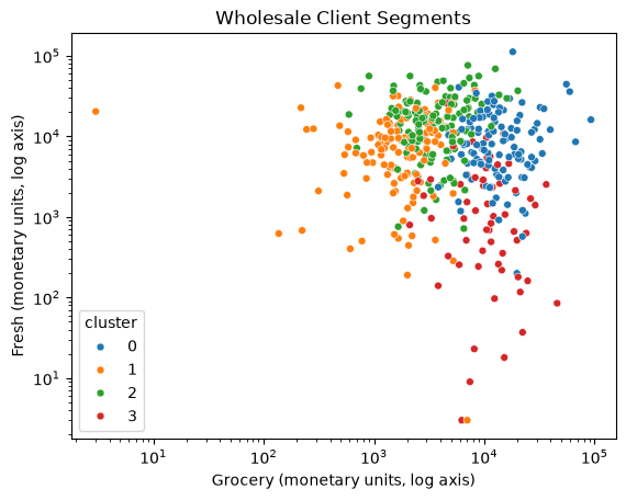
The plot shows only two of the six spending columns, so clusters that look close here may differ in the other four. The segments are best read from the profile tables. The channel column was not used to form the clusters, so it works as a side check on whether the segments make sense:
pd.crosstab(clients['cluster'], clients['channel'])
| channel | HoReCa | Retail |
|---|---|---|
| cluster | ||
| 0 | 25 | 94 |
| 1 | 129 | 1 |
| 2 | 123 | 7 |
| 3 | 21 | 40 |
From the profile tables and the channel counts, you can name each cluster and propose an action for it:
Cluster |
Profile |
Clients |
Possible action |
|---|---|---|---|
0 |
Household-goods retailers: grocery 12,311, detergents and paper 4,621 (5.7 times the overall median), milk 2.3 times; 94 of 119 are Retail |
119 |
Volume discounts on cleaning and paper goods and on grocery; consolidated deliveries |
1 |
Small accounts: below the overall median on milk, grocery, and detergents and paper, and near it on fresh food; 129 of 130 are HoReCa |
130 |
Low-cost service: standard catalog, fixed delivery days, a minimum order to keep deliveries worthwhile |
2 |
Fresh and frozen food service: fresh food 2.0 times and frozen food 2.8 times the overall median; 123 of 130 are HoReCa |
130 |
Frequent deliveries, reliable cold-chain service, supply contracts for fresh and frozen items |
3 |
Packaged-goods shops with little fresh food: fresh 0.13 and frozen 0.22 times the overall median, but milk, grocery, and detergents and paper far above it; 40 of 61 are Retail |
61 |
Bundles of dairy, grocery, and cleaning goods; no need for fresh-food logistics; check whether cafes in this group want a separate offer |
The channel counts support these names. Clusters 1 and 2 are almost entirely hotels, restaurants, and cafes, and cluster 0 is mostly retailers, but the clusters are not the channel. Cluster 3 mixes the two (21 HoReCa and 40 Retail clients), and clusters 0 and 3 buy similar amounts of packaged goods but very different amounts of fresh food, a distinction the channel label does not make.
These actions are hypotheses, not results. Before rolling one out, test it, for example with an A/B test that compares clients who get the offer with similar clients who don’t (Chapter 10). Also check that the segments are stable: if a different random start or a new year of data reshuffles the clients, the segments are not a solid basis for a decision.
### Exercise: Retail Share by Cluster
# Check whether clusters line up with the known sales channel.
#   1. For each cluster, compute the share of clients whose channel is 'Retail'.
#   2. Print the share for each cluster, rounded to 2 decimals.
# Print exactly:
# Cluster 0 Retail share: 0.67
# Cluster 1 Retail share: 0.25
import pandas as pd

ex_clients = pd.DataFrame({
    'cluster': [0, 0, 0, 1, 1, 1, 1],
    'channel': ['Retail', 'Retail', 'HoReCa', 'HoReCa', 'HoReCa', 'HoReCa', 'Retail'],
})
### Your code starts here.


### Your code ends here.
Cluster 0 Retail share: 0.67
Cluster 1 Retail share: 0.25
16.3.5. Practical Tips#
Scale features before clustering when units differ, and take logarithms first when the columns are heavily skewed, as spending columns usually are.
Run multiple initializations with
n_initto avoid poor local minima.Use
random_statefor reproducible examples.Treat cluster labels as arbitrary identifiers, not ranked categories.
Describe clusters in the original units, using medians when a few large values would distort the means.
If the silhouette score is low and no
kstands out, say so, and choosekfor the business use.Validate clusters with domain knowledge before using them for decisions.
16.3.6. Section Practice#
Use this short exercise to check the main workflow from this section.
### Exercise: Practice Interpreting Clusters
# K-means has assigned eight wholesale clients to clusters. Describe the clusters in business terms.
#   1. Use groupby to compute the median grocery and detergents_paper spending of each cluster.
#   2. Find the cluster with the highest median grocery spending and count its clients.
# Print exactly:
# Highest-grocery cluster: 2
# Median grocery: 11750.0
# Median detergents_paper: 4400.0
# Clients: 4
import pandas as pd

segments = pd.DataFrame({
    'grocery': [2100, 1800, 12500, 3200, 11000, 2600, 10500, 13000],
    'detergents_paper': [300, 250, 4600, 400, 4200, 350, 3100, 5200],
    'cluster': [0, 0, 2, 1, 2, 0, 2, 2],
})
### Your code starts here.


### Your code ends here.
Highest-grocery cluster: 2
Median grocery: 11750.0
Median detergents_paper: 4400.0
Clients: 4