

15.2. Evaluating Classifiers#
So far you have judged classifiers by one number, accuracy. Accuracy treats every mistake the same, but in business the two kinds of mistakes rarely cost the same. A bank that misses a fraudulent transaction loses the money; a bank that wrongly freezes a good customer’s card loses some goodwill and an hour of an analyst’s time. An online retailer that fails to nudge a visitor who was ready to buy may lose the sale; one that sends a coupon to a visitor who was never going to buy loses only the cost of the coupon.
This section introduces the standard tools for looking past accuracy: a baseline to compare against, the confusion matrix, precision and recall, and the cost of each kind of error. It continues with the real online shopping sessions (UCI Online Shoppers Purchasing Intention, introduced in Section Classification) and the same training and test sets as Section Nearest Neighbors with scikit-learn (the setup cell above recreates them), using the 11-nearest neighbor classifier chosen there on a validation set.
knn = make_pipeline(StandardScaler(), KNeighborsClassifier(n_neighbors=11))
knn.fit(X_train, y_train)
y_pred = knn.predict(X_test)

print('Test accuracy:', round(accuracy_score(y_test, y_pred), 3))
Test accuracy: 0.888
15.2.1. Why Accuracy Is Not Enough#
When one class is much more common than the other, the classes are imbalanced, and accuracy can look good even for a useless classifier. The simplest comparison is a baseline classifier that ignores the features and always predicts the majority class, the most common label in the training set. scikit-learn provides one as DummyClassifier.
baseline = DummyClassifier(strategy='most_frequent')
baseline.fit(X_train, y_train)
y_base = baseline.predict(X_test)

print('Baseline predicts:', y_base[0], 'for every session')
print('Baseline accuracy:', round(accuracy_score(y_test, y_base), 3))
print('kNN accuracy:     ', round(accuracy_score(y_test, y_pred), 3))
Baseline predicts: 0 for every session
Baseline accuracy: 0.845
kNN accuracy:      0.888
The baseline predicts “no purchase” (0) for every session and is right about 85% of the time, because about 85% of the test sessions do not end in a purchase. The classifier’s 89% accuracy is an improvement, but the honest gain is the difference between the two, about 4 percentage points, not the distance from 0%.
With rarer events the problem gets worse. Suppose a card issuer reviews 1,000 transactions, of which 20 (2%) are fraudulent. A “classifier” that approves everything is 98% accurate and catches no fraud at all.
actual_fraud = np.array([1] * 20 + [0] * 980)     # 1 = fraud, 0 = legitimate
approve_all = np.zeros(1000, dtype=int)           # predict "legitimate" for every transaction

print('Accuracy of approving everything:', accuracy_score(actual_fraud, approve_all))
print('Fraud cases caught:', np.sum((approve_all == 1) & (actual_fraud == 1)))
Accuracy of approving everything: 0.98
Fraud cases caught: 0
Accuracy alone cannot tell this useless rule apart from a good fraud detector. The two kinds of errors need to be counted separately.
### Exercise: Baseline for Loan Defaults
# A lender's test set has 400 loans, of which 48 defaulted (label 1).
# The counts are given below.
#   1. Compute the accuracy of always predicting "repaid" (0).
#   2. Compute the classifier's accuracy: it was right on 362 of the 400 loans.
#   3. Print how many percentage points the classifier beats the baseline by,
#      rounded to 1 decimal.
# Print exactly:
# Baseline accuracy: 0.88
# Classifier accuracy: 0.905
# Improvement (points): 2.5
ex_n_loans = 400
ex_n_default = 48
ex_n_correct = 362
### Your code starts here.


### Your code ends here.
Baseline accuracy: 0.88
Classifier accuracy: 0.905
Improvement (points): 2.5
15.2.2. The Confusion Matrix#
In a binary classification problem one class is called the positive class, usually the event you are trying to detect: a purchase, a default, fraud. “Positive” does not mean good; it means “the thing you are looking for”. Every prediction then falls into one of four groups:
Predicted positive (purchase) |
Predicted negative (no purchase) |
|
|---|---|---|
Actually positive (bought) |
True positive (TP): buyer correctly flagged |
False negative (FN): buyer missed |
Actually negative (did not buy) |
False positive (FP): non-buyer flagged by mistake |
True negative (TN): non-buyer correctly left alone |
A table of these four counts is called a confusion matrix, because it shows which classes the classifier confuses with each other. The correct predictions are on the diagonal (TN and TP); the two kinds of errors are off the diagonal.
You can count the groups yourself with pandas, using crosstab to cross-tabulate actual and predicted labels.
pd.crosstab(y_test, y_pred, rownames=['actual'], colnames=['predicted'])
| predicted | 0 | 1 |
|---|---|---|
| actual | ||
| 0 | 2969 | 158 |
| 1 | 255 | 317 |
scikit-learn’s confusion_matrix returns the same counts as an array, with actual classes as rows and predicted classes as columns, in the order 0, 1. For two classes, .ravel() flattens it into the four counts in the order TN, FP, FN, TP.
cm = confusion_matrix(y_test, y_pred)
print(cm)

tn, fp, fn, tp = cm.ravel()
print('TN:', tn, ' FP:', fp, ' FN:', fn, ' TP:', tp)
[[2969  158]
 [ 255  317]]
TN: 2969  FP: 158  FN: 255  TP: 317
ConfusionMatrixDisplay draws the matrix as a labeled picture, which is how it usually appears in reports.
fig, ax = plt.subplots(figsize=(4, 4))
ConfusionMatrixDisplay.from_predictions(
    y_test, y_pred, display_labels=['no purchase', 'purchase'], cmap='Blues', colorbar=False, ax=ax)
ax.grid(False)
plt.show()
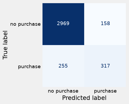
Of the 572 buyers in the test set, the classifier caught 317 (true positives) and missed 255 (false negatives). Of the 3,127 sessions without a purchase, it correctly left 2,969 alone (true negatives) and flagged 158 by mistake (false positives).
Accuracy is just the diagonal divided by the total:
print('Accuracy from the matrix:', round((tp + tn) / (tp + tn + fp + fn), 3))
Accuracy from the matrix: 0.888
### Exercise: Count the Four Outcomes
# A fraud model was checked on ten transactions (1 = fraud, the positive class).
#   1. Count the true positives, false positives, false negatives, and true negatives
#      by comparing ex_actual and ex_predicted.
#   2. Check your counts with confusion_matrix(ex_actual, ex_predicted).ravel().
# Print exactly:
# TP: 2 FP: 1 FN: 1 TN: 6
# sklearn: [6 1 1 2]
ex_actual = np.array([0, 0, 1, 0, 1, 0, 0, 1, 0, 0])
ex_predicted = np.array([0, 1, 1, 0, 0, 0, 0, 1, 0, 0])
### Your code starts here.


### Your code ends here.
TP: 2 FP: 1 FN: 1 TN: 6
sklearn: [6 1 1 2]
15.2.3. Precision, Recall, and F1#
Two summary rates answer the questions a manager actually asks about a flagging system.
Precision answers: of the sessions the classifier flagged, what fraction really ended in a purchase?
Recall (also called sensitivity) answers: of the sessions that really ended in a purchase, what fraction did the classifier catch?
Low precision means the marketing team spends coupons and attention on visitors who were never going to buy. Low recall means many buyers go unnoticed and get no nudge. The two usually pull against each other: flagging more sessions raises recall but tends to lower precision.
tn, fp, fn, tp = confusion_matrix(y_test, y_pred).ravel()

precision = tp / (tp + fp)
recall = tp / (tp + fn)

print('Precision:', round(precision, 3))
print('Recall:   ', round(recall, 3))
print('sklearn precision:', round(precision_score(y_test, y_pred), 3))
print('sklearn recall:   ', round(recall_score(y_test, y_pred), 3))
Precision: 0.667
Recall:    0.554
sklearn precision: 0.667
sklearn recall:    0.554
Precision is about 0.67: roughly two out of every three sessions the retailer flags really end in a purchase. Recall is about 0.55: the classifier catches about 55% of the buyers and misses the other 45%.
The always-“no purchase” baseline flags no one, so its recall is 0: it catches none of the buyers, which accuracy completely hid. (Its precision is undefined, since it makes no positive predictions; scikit-learn reports 0 and, with zero_division=0, does so without a warning.)
print('Baseline recall:   ', recall_score(y_test, y_base))
print('Baseline precision:', precision_score(y_test, y_base, zero_division=0))
Baseline recall:    0.0
Baseline precision: 0.0
When a single number is needed, the F1 score combines precision and recall. It is their harmonic mean, which is high only when both are high:
print('F1 by formula:', round(2 * precision * recall / (precision + recall), 3))
print('sklearn F1:   ', round(f1_score(y_test, y_pred), 3))
F1 by formula: 0.606
sklearn F1:    0.606
F1 is a convenient summary, but like accuracy it treats the two kinds of errors as equally important. When the costs of the errors are known, it is better to use them directly, as in the next subsection.
### Exercise: Precision and Recall for a Fraud Model
# A fraud model was checked on a month of transactions:
# it flagged 50 transactions, of which 30 were really fraud,
# and there were 40 fraudulent transactions in total.
#   1. Work out TP, FP, and FN from these facts.
#   2. Compute precision, recall, and F1, each rounded to 3 decimals.
# Print exactly:
# Precision: 0.6
# Recall: 0.75
# F1: 0.667
flagged = 50
flagged_and_fraud = 30
total_fraud = 40
### Your code starts here.


### Your code ends here.
Precision: 0.6
Recall: 0.75
F1: 0.667
15.2.4. The Business Cost of Errors#
To decide whether a classifier is worth using, put a dollar value on each kind of error. The data do not record costs, so the numbers below are assumptions made for this example, the kind of estimate a finance team would supply. Suppose the retailer plans to send every flagged session a nudge, a reminder email with free shipping, at a cost of about $3 per session.
False negative (a missed buyer): $30. Without a nudge, the retailer loses about $30 of profit it would have gained by closing the sale.
False positive (a flagged non-buyer): $3. The retailer pays for a nudge to someone who was not going to buy.
Together with a cost of zero for each correct prediction, these two numbers form a simple cost matrix: one cost for each cell of the confusion matrix.
To keep the arithmetic simple, assume that the nudge always secures the sale of a correctly flagged buyer, and count only the cost of the errors. (A fuller analysis would also count the cost of the nudges sent to true positives; the comparisons below would come out the same way, only with different totals.)
The total cost of the errors on the test set is
COST_FN = 30     # dollars lost for each buyer the model misses (an assumption)
COST_FP = 3      # dollars wasted for each non-buyer the model flags (an assumption)

def error_cost(actual, predicted):
    """Total dollar cost of the false negatives and false positives."""
    tn, fp, fn, tp = confusion_matrix(actual, predicted).ravel()
    return COST_FN * fn + COST_FP * fp

print('kNN cost:              $', error_cost(y_test, y_pred))
print('Baseline (flag no one): $', error_cost(y_test, y_base))
print('Flag everyone:          $', error_cost(y_test, np.ones(len(y_test), dtype=int)))
kNN cost:              $ 8124
Baseline (flag no one): $ 17160
Flag everyone:          $ 9381
The kNN classifier’s errors cost $8,124 on the 3,699 test sessions, less than half of the $17,160 lost by flagging no one, the baseline that looked 85% accurate. The third line is the surprise: flagging every session costs $9,381, only about $1,300 more than the classifier, even though its accuracy is just 15.5%. Because a missed buyer costs ten times as much as a false alarm, its 3,127 cheap false alarms cost far less than the baseline’s 572 expensive misses. Accuracy and cost can point in opposite directions: flagging everyone has the lowest accuracy of the three, yet the second-lowest cost.
The same reasoning applies to fraud. If a missed fraudulent transaction costs a bank an average of $500 and a false alarm costs $20 of an analyst’s review time, a classifier that catches more fraud can be worth many false alarms. The costs, not the accuracy, decide.
### Exercise: The Cost of a Fraud Model
# On 1,000 test transactions, a fraud model had TP = 15, FP = 40, FN = 5, TN = 940.
# A missed fraud (FN) costs $500 and a false alarm (FP) costs $20.
#   1. Compute the total error cost of the model.
#   2. Compute the error cost of approving everything (every fraud is missed: FN = 20, FP = 0).
# Print exactly:
# Model cost: 3300
# Approve-all cost: 10000
ex_tp, ex_fp, ex_fn, ex_tn = 15, 40, 5, 940
### Your code starts here.


### Your code ends here.
Model cost: 3300
Approve-all cost: 10000
15.2.5. Choosing Between Classifiers by Cost#
Once each error has a price, you can compare classifiers on the measure the business cares about. The table below evaluates nearest neighbor classifiers with several values of \(k\), plus the baseline, on accuracy, precision, recall, and total error cost.
(As in Section Nearest Neighbors with scikit-learn, a careful analyst would make this comparison on a validation set and use the test set only for the final report. The test set is used here to keep the example short.)
def evaluate(name, predicted):
    return {'classifier': name,
            'accuracy': round(accuracy_score(y_test, predicted), 3),
            'precision': round(precision_score(y_test, predicted, zero_division=0), 3),
            'recall': round(recall_score(y_test, predicted), 3),
            'error cost ($)': error_cost(y_test, predicted)}

rows = [evaluate('baseline (flag no one)', y_base),
        evaluate('flag everyone', np.ones(len(y_test), dtype=int))]
for k in [1, 5, 11, 21]:
    model = make_pipeline(StandardScaler(), KNeighborsClassifier(n_neighbors=k))
    model.fit(X_train, y_train)
    rows.append(evaluate(f'kNN, k = {k}', model.predict(X_test)))

comparison = pd.DataFrame(rows)
comparison
| classifier | accuracy | precision | recall | error cost ($) | |
|---|---|---|---|---|---|
| 0 | baseline (flag no one) | 0.845 | 0.000 | 0.000 | 17160 |
| 1 | flag everyone | 0.155 | 0.155 | 1.000 | 9381 |
| 2 | kNN, k = 1 | 0.854 | 0.526 | 0.554 | 8508 |
| 3 | kNN, k = 5 | 0.878 | 0.623 | 0.537 | 8508 |
| 4 | kNN, k = 11 | 0.888 | 0.667 | 0.554 | 8124 |
| 5 | kNN, k = 21 | 0.889 | 0.664 | 0.566 | 7932 |
Among the nearest neighbor classifiers, \(k = 21\) has both the highest accuracy (0.889) and the lowest cost ($7,932), with \(k = 11\) close behind (0.888 and $8,124). That agreement is not guaranteed; the exercise below gives a case where the more accurate model is the more expensive one. This section keeps \(k = 11\), the value chosen on the validation set in Section Nearest Neighbors with scikit-learn, because choosing \(k\) by looking at the test set would spoil it as a final check. Every one of these classifiers beats flagging everyone on cost, but only by about $900 to $1,450, a modest saving.
All of these classifiers predict “purchase” only when most of the neighbors ended in a purchase. Because a missed buyer costs ten times as much as a false alarm, it may pay to flag a session even when only a minority of similar sessions ended in a purchase. Changing that cutoff requires a classifier that reports a probability of purchase, which is where the next section begins.
### Exercise: Which Model Is Cheaper?
# Two models were checked on the same 300 test sessions.
#   Model A: FN = 30, FP = 10
#   Model B: FN = 12, FP = 60
#   1. Compute each model's accuracy (300 sessions in total) and error cost,
#      with a missed buyer costing $30 and a false alarm $3.
#   2. Print the name of the cheaper model.
# Print exactly:
# Model A: accuracy 0.867, cost 930
# Model B: accuracy 0.76, cost 540
# Cheaper: Model B
### Your code starts here.


### Your code ends here.
Model A: accuracy 0.867, cost 930
Model B: accuracy 0.76, cost 540
Cheaper: Model B