

16.4. Principal Component Analysis#
Note
Optional section. This section goes beyond the core clustering material in this chapter. The lab and homework do not use it. Read it if you want a tool for looking at data with many columns at once.
In K-Means Workflow you clustered the wholesale clients on two spending columns, so you could see every client on one scatter plot. The data have six spending columns, and real customer and product tables often have many more. Principal component analysis (PCA) is a way to summarize many correlated columns with a few new ones, so that you can plot the data, see its main patterns, and check what a clustering found.
16.4.1. Too Many Columns#
This section uses the wholesale clients again: 440 clients of a Portuguese distributor, from the UCI Machine Learning Repository (dataset 292, CC BY 4.0), as described in K-Means Workflow. This time it uses all six spending columns.
Feature |
Meaning |
|---|---|
|
Annual spending on fresh food |
|
Annual spending on milk and dairy products |
|
Annual spending on grocery items |
|
Annual spending on frozen food |
|
Annual spending on cleaning products and paper goods |
|
Annual spending on delicatessen items |
All amounts are in monetary units per year.
clients = pd.read_csv(path_data + 'wholesale_customers.csv')
clients.head()
| client_id | channel | region | fresh | milk | grocery | frozen | detergents_paper | delicatessen | |
|---|---|---|---|---|---|---|---|---|---|
| 0 | W001 | Retail | Other | 12669 | 9656 | 7561 | 214 | 2674 | 1338 |
| 1 | W002 | Retail | Other | 7057 | 9810 | 9568 | 1762 | 3293 | 1776 |
| 2 | W003 | Retail | Other | 6353 | 8808 | 7684 | 2405 | 3516 | 7844 |
| 3 | W004 | HoReCa | Other | 13265 | 1196 | 4221 | 6404 | 507 | 1788 |
| 4 | W005 | Retail | Other | 22615 | 5410 | 7198 | 3915 | 1777 | 5185 |
Each client is now a point in six dimensions. The number of features is the data’s dimensionality. You cannot draw a six-dimensional scatter plot. You could draw a scatter plot for every pair of features, but six features give 15 pairs, and none of them shows the whole picture.
The features also overlap. Clients that buy a lot of groceries tend to buy a lot of cleaning and paper goods too. The correlation table (correlation was introduced in Chapter 12) shows how strongly each pair of features moves together. As in K-Means Workflow, take base-10 logarithms of the spending first, because a few very large clients would otherwise dominate the correlations:
spend_cols = ['fresh', 'milk', 'grocery', 'frozen', 'detergents_paper', 'delicatessen']
X = np.log10(clients[spend_cols])

plt.figure(figsize=(7, 5.5))
sns.heatmap(X.corr(), annot=True, fmt='.2f', cmap='RdBu_r', vmin=-1, vmax=1)
plt.title('Correlations Between Log Spending Columns')
plt.show()
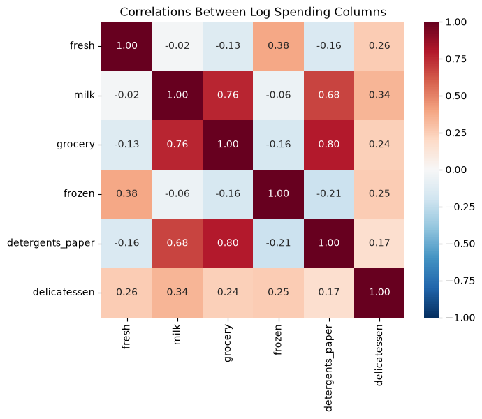
Grocery and detergents and paper have a correlation of 0.80, the highest of the 15 pairs, so they carry much of the same information: knowing a client’s spending on one tells you a lot about the other. Milk is also strongly related to both (0.76 with grocery and 0.68 with detergents and paper). Fresh and frozen food are only weakly related to these three, and fresh and frozen food are moderately related to each other (0.38). When columns overlap like this, the data have fewer independent patterns than they have columns.
Dimensionality reduction means replacing many features with a few new ones that keep most of the information. PCA is the most common method for numeric data.
### Exercise: Find the Most Correlated Pair
# Use the wholesale clients data with log10 spending.
#   1. Take the base-10 logarithm of the six spending columns and compute their correlation table.
#   2. Find the correlation between grocery and detergents_paper.
#   3. Find the correlation between fresh and frozen.
# Print each correlation rounded with round(..., 2).
# Print exactly:
# grocery vs detergents: 0.8
# fresh vs frozen: 0.38
import numpy as np
import pandas as pd

ex_clients = pd.read_csv(path_data + 'wholesale_customers.csv')
ex_spend_cols = ['fresh', 'milk', 'grocery', 'frozen', 'detergents_paper', 'delicatessen']
### Your code starts here.


### Your code ends here.
grocery vs detergents: 0.8
fresh vs frozen: 0.38
16.4.2. Principal Components as New Axes#
Start with just two features that move together, grocery and detergents and paper. Put both (after the logarithm) in standard units first (Chapter 12), so that each is measured in standard deviations from its mean, as you did for clustering in the previous section.
two = np.log10(clients[['grocery', 'detergents_paper']])
two_su = (two - two.mean()) / two.std(ddof=0)      # standard units

pca_two = PCA(n_components=2)
pca_two.fit(two_su)

direction = pca_two.components_[0]     # direction of the first component
direction
array([0.70710678, 0.70710678])
A principal component is a new axis through the data. The first principal component, PC1, points in the direction in which the data are most spread out. components_[0] holds that direction: it moves about 0.71 standard units in detergents and paper for every 0.71 standard units in grocery, so it runs diagonally through the cloud of points. (The signs of both numbers could be reversed; this comes up again below.) The second component, PC2, is at a right angle to PC1 and picks up the spread that is left over.
The plot on the left draws both axes on the scatter plot. The plot on the right shows the same clients measured on the new axes: PCA has simply rotated the axes so that the long direction of the cloud lies along the horizontal axis.
scores_two = pca_two.transform(two_su)     # each client's position on PC1 and PC2

fig, axes = plt.subplots(1, 2, figsize=(11, 4.5))

axes[0].scatter(two_su['grocery'], two_su['detergents_paper'], alpha=0.5)
for i, name in enumerate(['PC1', 'PC2']):
    d = pca_two.components_[i] * 2.2
    axes[0].annotate('', xy=d, xytext=(0, 0),
                     arrowprops=dict(arrowstyle='->', color='crimson', lw=2))
    axes[0].text(d[0] * 1.1, d[1] * 1.1, name, color='crimson', fontsize=12)
axes[0].set_xlabel('Grocery (log10, standard units)')
axes[0].set_ylabel('Detergents and paper (log10, standard units)')
axes[0].set_title('Original axes')
axes[0].set_xlim(-3.6, 3.6)
axes[0].set_ylim(-3.6, 3.6)
axes[0].set_aspect('equal')

axes[1].scatter(scores_two[:, 0], scores_two[:, 1], alpha=0.5)
axes[1].set_xlabel('PC1')
axes[1].set_ylabel('PC2')
axes[1].set_title('Rotated axes')
axes[1].set_aspect('equal')

plt.tight_layout()
plt.show()
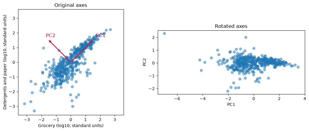
Most of the spread now runs along PC1, and the points vary only a little along PC2. The model reports how much of the total spread each component captures:
pca_two.explained_variance_ratio_
array([0.89819887, 0.10180113])
PC1 captures about 90% of the variation in the two features, and PC2 only about 10%. One number per client, the PC1 score, which you could call “household-goods spending”, keeps almost all of what grocery and detergents and paper spending tell you. That is the idea of PCA: when features overlap, a few well-chosen directions can replace many columns.
### Exercise: PCA on Two Features
# A manager wants one "fresh and frozen" measure built from the fresh and frozen columns.
#   1. Take log10 of the two columns and put them in standard units.
#   2. Fit PCA with 2 components.
#   3. Print the share of variation captured by PC1, rounded to 2 decimal places.
# Print exactly:
# PC1 share: 0.69
import numpy as np
import pandas as pd
from sklearn.decomposition import PCA

ex_clients = pd.read_csv(path_data + 'wholesale_customers.csv')
pair = np.log10(ex_clients[['fresh', 'frozen']])
### Your code starts here.


### Your code ends here.
PC1 share: 0.69
16.4.3. Standardize, Then Fit PCA#
PCA looks for the directions with the most spread, so, like k-means, it depends on the units and the skew of the features. In monetary units, the standard deviation of fresh spending is about 12,600, while that of delicatessen is about 2,800, and a few clients spend many times the typical amount. Here is PCA on the raw features:
pca_raw = PCA().fit(clients[spend_cols])
pd.Series(pca_raw.components_[0], index=spend_cols).round(3)
fresh               0.977
milk                0.121
grocery             0.062
frozen              0.152
detergents_paper   -0.007
delicatessen        0.068
dtype: float64
pca_raw.explained_variance_ratio_[0]
np.float64(0.45961361681363955)
On the raw features, PC1 is almost exactly fresh (weight about 0.98, the others 0.15 or less) and claims about 46% of the variation, only because fresh spending has the largest numbers. As with k-means, take logarithms and put the features in standard units, so that each feature starts with the same spread:
X_scaled = pd.DataFrame(StandardScaler().fit_transform(X), columns=spend_cols)   # standard units

pca = PCA()            # keep all 6 components for now
pca.fit(X_scaled)

pca.explained_variance_ratio_.round(3)
array([0.44 , 0.271, 0.108, 0.101, 0.049, 0.031])
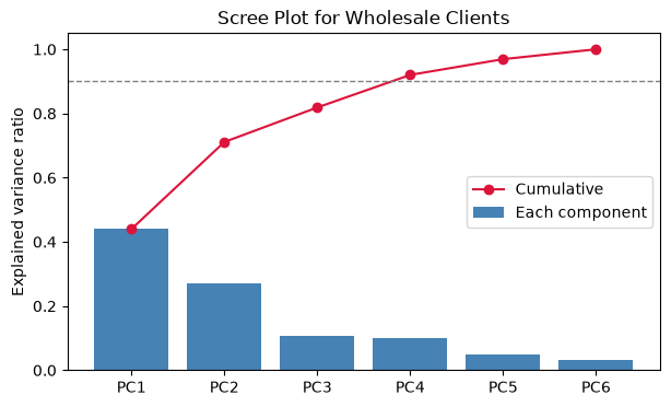
The explained variance ratio of a component is the share of the total variation in the scaled data that the component captures. The ratios are in order from largest to smallest and add up to 1. A scree plot shows them as bars, often with the running (cumulative) total as a line:
ratios = pca.explained_variance_ratio_
pcs = [f'PC{i}' for i in range(1, len(ratios) + 1)]

plt.figure(figsize=(7, 4))
plt.bar(pcs, ratios, color='steelblue', label='Each component')
plt.plot(pcs, ratios.cumsum(), color='crimson', marker='o', label='Cumulative')
plt.axhline(0.9, color='gray', linestyle='--', linewidth=1)
plt.ylim(0, 1.05)
plt.ylabel('Explained variance ratio')
plt.title('Scree Plot for Wholesale Clients')
plt.legend()
plt.show()
pd.DataFrame({'component': pcs,
              'explained': ratios.round(3),
              'cumulative': ratios.cumsum().round(3)})
| component | explained | cumulative | |
|---|---|---|---|
| 0 | PC1 | 0.440 | 0.440 |
| 1 | PC2 | 0.271 | 0.711 |
| 2 | PC3 | 0.108 | 0.819 |
| 3 | PC4 | 0.101 | 0.920 |
| 4 | PC5 | 0.049 | 0.969 |
| 5 | PC6 | 0.031 | 1.000 |
Choosing how many components to keep. PC1 captures about 44% of the variation, PC2 about 27%, and PC3 about 11%. After PC2 the bars drop and then shrink slowly: PC3 and PC4 hold about 11% and 10%, and PC5 and PC6 together hold about 8%. Three common rules of thumb:
Keep the components before the scree plot levels off (the “elbow”, as with choosing k in the previous section). Here the bars drop steeply after PC1 and again after PC2, then nearly level off (PC3 and PC4 are about equal), so the elbow suggests two, though it is not sharp.
Keep enough components to reach a target share, such as 80% or 90%. Here, three components reach about 82% and four reach about 92%.
For a picture, keep two. PC1 and PC2 together hold about 71% of the variation, enough to show the main patterns on one scatter plot.
As with choosing k, these are guides. The right number depends on what the components will be used for. Six columns do not shrink as much as a table with dozens of overlapping columns would, because these six are only partly correlated.
### Exercise: How Many Components?
# Use ex_X_scaled, the six wholesale spending columns after log10 and standardizing.
#   1. Fit PCA with all components.
#   2. Compute the cumulative explained variance ratio.
#   3. Find the smallest number of components whose cumulative share is at least 0.85.
# Print exactly:
# Components needed: 4
import numpy as np
import pandas as pd
from sklearn.decomposition import PCA

ex_clients = pd.read_csv(path_data + 'wholesale_customers.csv')
ex_spend_cols = ['fresh', 'milk', 'grocery', 'frozen', 'detergents_paper', 'delicatessen']
ex_X = np.log10(ex_clients[ex_spend_cols])
ex_X_scaled = (ex_X - ex_X.mean()) / ex_X.std(ddof=0)
### Your code starts here.


### Your code ends here.
Components needed: 4
16.4.4. Reading the Loadings#
A component is a weighted combination of the original features. The weights are called loadings, and they are stored in components_, one row per component. A large positive loading means the feature rises with the component; a large negative loading means it falls; a loading near 0 means the feature has little to do with that component.
loadings = pd.DataFrame(pca.components_[:3].T, index=spend_cols,
                        columns=['PC1', 'PC2', 'PC3'])
loadings.round(2)
| PC1 | PC2 | PC3 | |
|---|---|---|---|
| fresh | -0.10 | 0.59 | -0.63 |
| milk | 0.54 | 0.13 | -0.08 |
| grocery | 0.57 | -0.01 | -0.13 |
| frozen | -0.14 | 0.59 | -0.03 |
| detergents_paper | 0.55 | -0.07 | -0.20 |
| delicatessen | 0.21 | 0.53 | 0.73 |
fig, axes = plt.subplots(1, 2, figsize=(11, 4), sharey=True)
for ax, pc in zip(axes, ['PC1', 'PC2']):
    sns.barplot(x=loadings[pc], y=loadings.index, ax=ax, color='steelblue')
    ax.axvline(0, color='black', linewidth=0.8)
    ax.set_title(f'Loadings on {pc}')
    ax.set_xlabel('Loading')
plt.tight_layout()
plt.show()
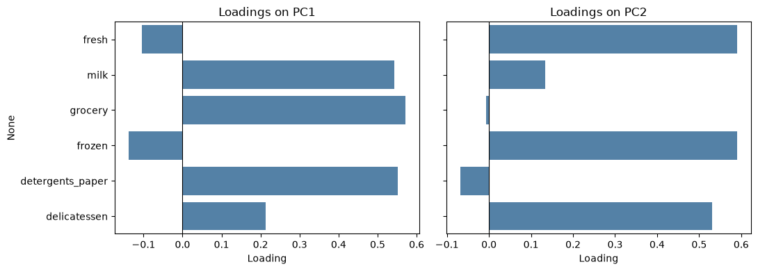
Read each component by looking for the features with the largest loadings, positive and negative:
PC1: grocery (0.57), detergents and paper (0.55), and milk (0.54) are high, and fresh (-0.10) and frozen (-0.14) are slightly negative. A client scores high on PC1 by spending a lot on packaged household goods. You might name PC1 household and packaged goods.
PC2: fresh (0.59), frozen (0.59), and delicatessen (0.53) are high, while milk (0.13), grocery (-0.01), and detergents and paper (-0.07) are near zero. A client scores high on PC2 by spending a lot on fresh, frozen, and delicatessen food. You might name PC2 fresh and prepared food.
PC3 contrasts delicatessen (0.73) with fresh food (-0.63): a client scores high by spending more on delicatessen than on fresh food. It holds a smaller share of the variation than the first two.
PC1 and PC2 describe two different kinds of buying, and the fact that they are separate is the point: spending on household goods and spending on food are close to independent across the distributor’s clients.
Caution
The names are an interpretation, not something PCA computes. Two analysts can read the same loadings and choose different names. The sign of a component is also arbitrary: another version of scikit-learn could flip PC1 so that all its loadings change sign, which would turn “high on household goods” into “low on household goods” without changing anything about the data. Always check the loadings before you name a component, and say which features drive it when you present it.
### Exercise: Read the Loadings
# Use the loadings table for the six scaled spending columns.
#   1. Fit PCA with 3 components on ex_X_scaled and build a table of loadings (features as rows).
#   2. Find the feature with the largest absolute loading on PC3.
# Print exactly:
# Largest PC3 loading: delicatessen
import numpy as np
import pandas as pd
from sklearn.decomposition import PCA

ex_clients = pd.read_csv(path_data + 'wholesale_customers.csv')
ex_spend_cols = ['fresh', 'milk', 'grocery', 'frozen', 'detergents_paper', 'delicatessen']
ex_X = np.log10(ex_clients[ex_spend_cols])
ex_X_scaled = (ex_X - ex_X.mean()) / ex_X.std(ddof=0)
### Your code starts here.


### Your code ends here.
Largest PC3 loading: delicatessen
16.4.5. PCA with Clustering#
PCA and k-means work well together. Cluster the clients on all six scaled features, exactly as in the previous section, and then use PCA to draw the result. First, a quick silhouette check for the number of clusters:
for k in range(2, 8):
    labels = KMeans(n_clusters=k, n_init=10, random_state=101).fit_predict(X_scaled)
    print(k, round(silhouette_score(X_scaled, labels), 3))
2 0.29
3 0.258
4 0.188
5 0.196
6 0.199
7 0.184
As in the previous section, the silhouette score is highest at k = 2 (about 0.29) and about the same, 0.18 to 0.20, for k = 4 to 7. No k stands out, so keep the choice of k = 4 from the previous section. Fit k-means with 4 clusters and plot each client at its PC1 and PC2 scores, colored by cluster:
kmeans = KMeans(n_clusters=4, n_init=10, random_state=101)
clients['cluster'] = kmeans.fit_predict(X_scaled)

scores = pca.transform(X_scaled)          # PC scores for every client
clients['PC1'] = scores[:, 0]
clients['PC2'] = scores[:, 1]

sns.scatterplot(data=clients, x='PC1', y='PC2', hue='cluster', palette='tab10')
plt.xlabel('PC1: household and packaged goods')
plt.ylabel('PC2: fresh and prepared food')
plt.title('Wholesale Segments on the First Two Components')
plt.show()
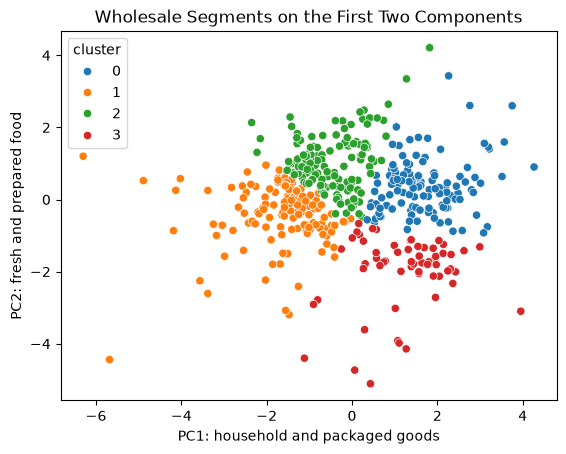
Six features are now one picture. The four segments occupy different regions of the plot, though they touch where the clients are in between: the clients form a continuous cloud, as the silhouette scores showed. The axis names come from the loadings, so the picture already suggests what each segment is: high or low on household goods, high or low on fresh and prepared food. To describe the segments, though, go back to the original units, as in the previous section. A manager can act on monetary units, not on PC scores.
profile = clients.groupby('cluster')[spend_cols].median().round(0)
profile['clients'] = clients['cluster'].value_counts().sort_index()
profile
| fresh | milk | grocery | frozen | detergents_paper | delicatessen | clients | |
|---|---|---|---|---|---|---|---|
| cluster | |||||||
| 0 | 7842.0 | 8384.0 | 12311.0 | 1365.0 | 4621.0 | 1682.0 | 119 |
| 1 | 7814.0 | 1112.0 | 1820.0 | 1386.0 | 224.0 | 432.0 | 130 |
| 2 | 16978.0 | 3122.0 | 3430.0 | 4324.0 | 515.0 | 1374.0 | 130 |
| 3 | 1073.0 | 6964.0 | 10518.0 | 340.0 | 4508.0 | 295.0 | 61 |
The profiles match the picture, and they are the same four segments as in the previous section. One cluster buys a lot of milk, grocery, and detergents and paper (household-goods retailers, high on PC1). One buys little milk, grocery, or cleaning goods (small accounts, low on PC1). One buys the most fresh and frozen food (fresh and frozen food service, high on PC2). One buys household goods but almost no fresh or frozen food (packaged-goods shops, high on PC1 and low on PC2). As before, the cluster numbers themselves are arbitrary.
PCA for visualization vs. PCA before clustering. Above, k-means used all six features, and PCA only drew the result. Another option is to reduce the data first and cluster the PC scores. This can help when there are many noisy or overlapping features, and it makes the clusters easier to plot. But the clusters then ignore whatever the dropped components held; here, clustering only PC1 and PC2 would ignore the 29% of the variation in PC3 to PC6, including the contrast between delicatessen and fresh food. Compare the two:
labels_2pc = KMeans(n_clusters=4, n_init=10, random_state=101).fit_predict(scores[:, :2])
table = pd.crosstab(clients['cluster'], labels_2pc, rownames=['all 6 features'], colnames=['first 2 PCs'])
print(table)

same = table.max(axis=1).sum()      # clients in the best-matching group of each row
print('Clients grouped the same way, ignoring the names:', same, 'of', len(clients))
first 2 PCs      0    1    2    3
all 6 features
0                7    0    5  107
1                1  127    2    0
2                0    2  126    2
3               61    0    0    0
Clients grouped the same way, ignoring the names: 421 of 440
Each row has one large count, so the two approaches put most clients in the same group (the cluster numbers differ, but the groups largely agree). They agree on 421 of 440 clients (96%), and the 19 that differ sit between groups. That is because the first two components hold most of the variation, and the segments differ mostly on household goods and on fresh and frozen food. With more columns or more complex data the two approaches often disagree more, so report which one you used.
### Exercise: Cluster the PC Scores
# Use the PC scores of the six scaled wholesale spending columns.
#   1. Fit PCA on ex_X_scaled and keep the first 3 components' scores.
#   2. Fit KMeans with 4 clusters (n_init=10, random_state=101) on those scores.
#   3. Print the cluster sizes sorted from smallest to largest, as a list.
# Print exactly:
# Cluster sizes: [69, 110, 116, 145]
import numpy as np
import pandas as pd
from sklearn.decomposition import PCA
from sklearn.cluster import KMeans

ex_clients = pd.read_csv(path_data + 'wholesale_customers.csv')
ex_spend_cols = ['fresh', 'milk', 'grocery', 'frozen', 'detergents_paper', 'delicatessen']
ex_X = np.log10(ex_clients[ex_spend_cols])
ex_X_scaled = (ex_X - ex_X.mean()) / ex_X.std(ddof=0)
### Your code starts here.


### Your code ends here.
Cluster sizes: [69, 110, 116, 145]
16.4.6. Limits of PCA#
PCA is a useful first look at data with many columns, but keep its limits in mind:
Linear only. Each component is a straight-line direction, a weighted sum of the features. Curved or more complex patterns may not show up in the first few components.
Sensitive to scaling. As you saw, PCA on raw features is dominated by whichever feature has the biggest numbers, here fresh food. Standardize first unless the features already share a unit, and take logarithms when a few very large values stretch a column.
Harder to explain. “PC1 score of 1.8” means nothing to a manager until you translate it into the features that drive it. Original columns such as grocery and fresh are easier to explain, so present results in the original units and use components as a summary or a map.
Spread is not importance. PCA keeps the directions with the most variation, which are not always the ones that matter for a decision. A small component can still hold the signal that predicts churn or profit.
Numeric features. PCA works with numeric columns. Categories such as channel or region need other methods.